Notebook · 2021
MNIST Classification
MNIST Classification with Gradient Descent.ipynb
Notebook SHA-256 4d76eabe8aa8 · 104 cells · 25 figures
Saved outputs shown as found. The notebook was not re-executed. No local paths or credential patterns were found.
MNIST Classification with Gradient Descent and its variants
by Vrinda Chauhan
Python libraries
We will use the following Python libraries to analyze this dataset:
- pandas: dataframe data structure based on the the naive R data structure. Some advantages of using this library is that it utilizes vectorized processes for fast manipulation of the data. In terms of memory usage, however, pandas is much less efficient; its advantage lies in computations for datasets larger than 500,000 rows
- numpy: python library that allows us to perform various mathematical operationss, especially for constructing and working with multidimensional arrays. numpy is better for memory usage for datasets smaller than 50,000 rows, and it allows use to use list comprehension instead of loops for our operations.
- matplotlib: 2d plotting tools
- IPython.display: displays the dataframes in a clean way
- time: allows us to record and then calculate the speed of the different algorithms
In [1]
import pandas as pd
import numpy as np
import matplotlib.pyplot as plt
from IPython.display import display, HTML
from time import time
%matplotlib inline
Discussion of the dataset
The MNIST dataset is a dataset of handwritten digits and their corresponding pixels. The data is split into two different datasets, one of the training data and one of the test data.
The first column of each data record is the label of the handwritten digit, a number from 0-9. The rest of the data record consists of the values of the pixels of the digit, a number between 0 and 255. This segment is a vector $x_{i} \in R^{784}$, which are concatinated from an image of $28x28$ pixels of the given digit.
Let's see what this looks like.
In [2]
train = pd.read_csv('./mnist_train.csv', header=None)
In [3]
test = pd.read_csv('./mnist_test.csv', header=None)
In [4]
print('The size of the training data is ', train.shape)
print('The size of the test data is ', test.shape)
The size of the training data is  (60000, 785)
The size of the test data is  (10000, 785)
In [5]
display(HTML(train.head(15).to_html()))
| 0 | 1 | 2 | 3 | 4 | 5 | 6 | 7 | 8 | 9 | 10 | 11 | 12 | … | |
|---|---|---|---|---|---|---|---|---|---|---|---|---|---|---|
| 0 | 5 | 0 | 0 | 0 | 0 | 0 | 0 | 0 | 0 | 0 | 0 | 0 | 0 | … |
| 1 | 0 | 0 | 0 | 0 | 0 | 0 | 0 | 0 | 0 | 0 | 0 | 0 | 0 | … |
| 2 | 4 | 0 | 0 | 0 | 0 | 0 | 0 | 0 | 0 | 0 | 0 | 0 | 0 | … |
| 3 | 1 | 0 | 0 | 0 | 0 | 0 | 0 | 0 | 0 | 0 | 0 | 0 | 0 | … |
| 4 | 9 | 0 | 0 | 0 | 0 | 0 | 0 | 0 | 0 | 0 | 0 | 0 | 0 | … |
| 5 | 2 | 0 | 0 | 0 | 0 | 0 | 0 | 0 | 0 | 0 | 0 | 0 | 0 | … |
| 6 | 1 | 0 | 0 | 0 | 0 | 0 | 0 | 0 | 0 | 0 | 0 | 0 | 0 | … |
| 7 | 3 | 0 | 0 | 0 | 0 | 0 | 0 | 0 | 0 | 0 | 0 | 0 | 0 | … |
| 8 | 1 | 0 | 0 | 0 | 0 | 0 | 0 | 0 | 0 | 0 | 0 | 0 | 0 | … |
| 9 | 4 | 0 | 0 | 0 | 0 | 0 | 0 | 0 | 0 | 0 | 0 | 0 | 0 | … |
| 10 | 3 | 0 | 0 | 0 | 0 | 0 | 0 | 0 | 0 | 0 | 0 | 0 | 0 | … |
| 11 | 5 | 0 | 0 | 0 | 0 | 0 | 0 | 0 | 0 | 0 | 0 | 0 | 0 | … |
Showing 12 of 15 rows and 14 of 786 columns. Full data is in the source notebook.
In [6]
display(HTML(test.head(15).to_html()))
| 0 | 1 | 2 | 3 | 4 | 5 | 6 | 7 | 8 | 9 | 10 | 11 | 12 | … | |
|---|---|---|---|---|---|---|---|---|---|---|---|---|---|---|
| 0 | 7 | 0 | 0 | 0 | 0 | 0 | 0 | 0 | 0 | 0 | 0 | 0 | 0 | … |
| 1 | 2 | 0 | 0 | 0 | 0 | 0 | 0 | 0 | 0 | 0 | 0 | 0 | 0 | … |
| 2 | 1 | 0 | 0 | 0 | 0 | 0 | 0 | 0 | 0 | 0 | 0 | 0 | 0 | … |
| 3 | 0 | 0 | 0 | 0 | 0 | 0 | 0 | 0 | 0 | 0 | 0 | 0 | 0 | … |
| 4 | 4 | 0 | 0 | 0 | 0 | 0 | 0 | 0 | 0 | 0 | 0 | 0 | 0 | … |
| 5 | 1 | 0 | 0 | 0 | 0 | 0 | 0 | 0 | 0 | 0 | 0 | 0 | 0 | … |
| 6 | 4 | 0 | 0 | 0 | 0 | 0 | 0 | 0 | 0 | 0 | 0 | 0 | 0 | … |
| 7 | 9 | 0 | 0 | 0 | 0 | 0 | 0 | 0 | 0 | 0 | 0 | 0 | 0 | … |
| 8 | 5 | 0 | 0 | 0 | 0 | 0 | 0 | 0 | 0 | 0 | 0 | 0 | 0 | … |
| 9 | 9 | 0 | 0 | 0 | 0 | 0 | 0 | 0 | 0 | 0 | 0 | 0 | 0 | … |
| 10 | 0 | 0 | 0 | 0 | 0 | 0 | 0 | 0 | 0 | 0 | 0 | 0 | 0 | … |
| 11 | 6 | 0 | 0 | 0 | 0 | 0 | 0 | 0 | 0 | 0 | 0 | 0 | 0 | … |
Showing 12 of 15 rows and 14 of 786 columns. Full data is in the source notebook.
Note the data will be normalized, ie divided by 255 so that each pixel entry will be a real number in $[0,1]$; this is mainly to simplify the mathematical calculations in the gradient or loss, for example.
Visualizing MNIST Digits
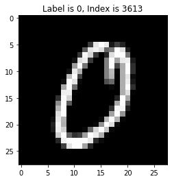
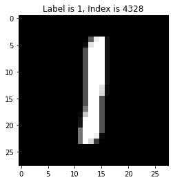
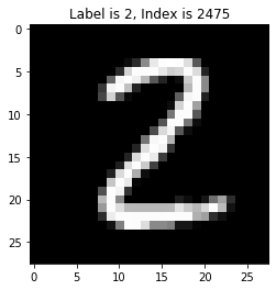
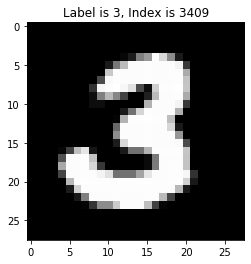
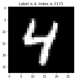
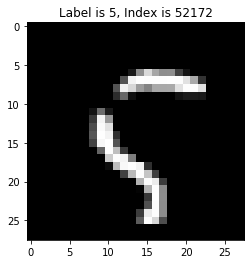
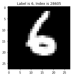
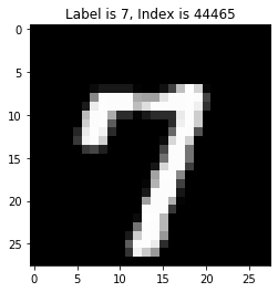
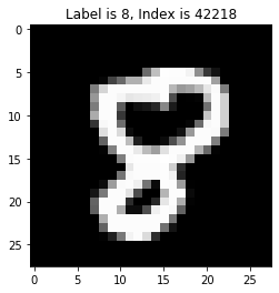
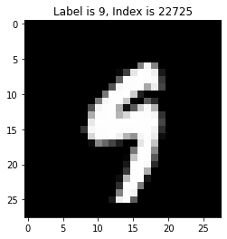
We mentioned earlier that each data record has a label and a concatinated pixel vector. Let's try to visualize what a randomly chosen digit from the training set will look like for each digit. To do this, we can define the following helper function:
In [7]
def visualize(df, i):
    ''''
    This method helps us visualize the digits from their concatinated vector as a row of the dataset into the image it
    represents.
    Parameters: a dataset df, a desired digit we want to visualize, i
    Output: a plot with the digit and the corresponding index, chosen randomly
    '''
    a = df[df.columns[0]]
    label = list((float(i) for i in (a)))
    # n is our on and off switch for the while loop
    n = 0
    # the while loop picks a randomly indexed data record chosen by the np.random.choice method and compares its label
    # to our desired i; if it is our desired digit then we engage in plotting it. If not, we keep remain engaged in the
    # while loop to keep picking random indexes
    while (n == 0):
        a_choice = np.random.choice(range(n, len(label)))
        if i == label[a_choice]:
            a_pixels = df.loc[a_choice]
            a_pixels = np.array(a_pixels[1:], dtype='uint8')
            a_pixels = a_pixels.reshape((28, 28))
            plt.imshow(a_pixels, cmap='gray')
            plt.title('Label is {i}, Index is {a_choice}'.format(
                i=i, a_choice=a_choice))
            plt.show()
            n = 1
        else:
            n = 0
In [8]
visualize(test, 0)
visualize(test, 1)
visualize(test, 2)
visualize(test, 3)
visualize(test, 4)
visualize(train, 5)
visualize(train, 6)
visualize(train, 7)
visualize(train, 8)
visualize(train, 9)
Discussion of the problem
With this dataset, we want to solve a classification problem using discriminant analysis; that is, we want an algorithm to be able to recognize the digit of an input pixel vector between a set of two digits in 0-9. We want to use the training sample to find a vector such that when we take the cross product of a data record's pixel segment and a derived weight vector, we can predict which digit the pixel vector represents between two given digits (in the algorithm, we correspond each of these digits with 1, -1 to make this calculation and function easier). In mathematical terms, we want $w$ such that $$ y_{i} = sign(w^{T}x_{i}) $$ where y is the label for the $i^{th}$ data record and the $x_{i}$ is the vector of pixels for that digit. Intuitively, what we are looking for the best fitting hyperplane that serperates the class of one digit's pixels from the class of the other digit's pixels. This will allow us to have a vector that makes predictions for the test data. In 2-D (ie if the data only had two columns), this idea can be illustrated by the following image: !image.png Here, the dots are 2-d datapoints, and we want to find the line that best seperates the two clusters of data. Recall the function of a line is $ y = mx + b$, so in 2-D, our "weight vector" is the variable $m$, and we would want to pick or "learn" an $m$ so that the distances of the dotted lines are minimized.
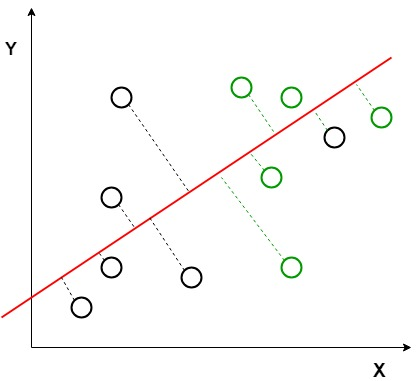
Since our dataset has 784 columns, we want to try to learn a length 784 weight vector so that we can seperate the two classes of data and make predictions on the test set. Using this, we can understand and compare the performance of each model to assess the accuracy, speed, and computational complexity of the model, and understand the different tradeoffs made in each method. We will use the gradient descent algorithm and its variations to solve this problem.
Discussion of the various Gradient Descent Methods
Discussion of the loss function and some probability
In order to understand the gradient descent algorithm, we must first understand the distribution of the dataset, and the loss function affiliated with it. A loss function calculates the error rate for the classification. Our goal is to minimize this loss function.
In the MNIST dataset, we will be using a loss function called cross-entropy loss, which we will derive below.
It can be shown the cumilitive distribution function of $G_{z}(z) = \frac{1}{1+e^{-z}} $ can model the probability of a given digit being the correct class label, if we affiliate our labels with a -1 and 1 (for example, if our model was meant to decide if a set of pixels is a 4 or 9, we could affiliate 4 with the "1" value and 9 with the "-1" value).
Consider the random variable $y := sign(\alpha + z)$ for $z$ as with the CDF, $\alpha$ fixed (we will discuss shortly how $\alpha$ is chosen). To see that $G_{z}(z)$ works here as a CDF, we can write $P(y= 1)$ and $P(y= -1)$ in terms of the CDF. $P(y=1)$ can be rewritten as $P(z > - \alpha)$ since $y=1$ when $\alpha + z > 0$ or $z > -\alpha$. Thus, we can use the CDF to solve this, by writing $$P(y=1) = P(z > - \alpha) = 1-G_{z}(-a) = 1- \frac{1}{1+e^{-(-\alpha)}} = 1 - \frac{1}{1+e^{\alpha}}= \frac{e^{\alpha}}{1+e^{\alpha}}= \frac{1}{1+e^{-\alpha}} $$
Similarly, for $P(y=-1)$, we evaluate $P(z < -a)$ since $y<0$ when $\alpha + z < 0$, or $z < -\alpha$. Thus we can write $$P(y = -1) = P(z < -\alpha) = G_Z(-a)= \frac{1}{1+e^{\alpha}}$$
From this, it is plain to see what the probability mass function for y is $P(y) = \frac{1}{1+e^{-\alpha y}} $, and for multiple $y$'s that are independent and identically distributed (as we have with the labels for MNIST data) we can write this as $P(y) = \prod_{i=1}^{N} \frac{1}{1+e^{-\alpha_{i} y_{i}}} $ for a fixed set of $\alpha_{i}'s$.
Now that we have done some groundwork for our loss function, we can discuss how $\alpha_{i}'s$ are chosen. In our MNIST dataset, if we set $\alpha_{i} = w^{T}x_{i}$ for $x_{i}$ being the pixel vector for the $i^{th}$ data record, we can solve our classification problem by maximizing the resulting function. This function would look like $$H(w) = \prod_{i=1}^{N} \frac{1}{1+e^{-w^{T}x_{i} y_{i}}} $$.
So why does maximizing $H(w)$ solve our problem? We want to maximize $H(w)$ because this will give us the probability that the parities of $w^Tx_i$ and $y_i$ match. Indeed if the parities differ, then $w^{T}x_{i} y_{i}$ would be a negative expression, which would cancel with the negative inside the function, so $H(w)$ would simplify to $\frac{1}{1+e^{w^T x_i y_i}}$, which makes $e^{w^T x_i y_i}$ large, and the overall expression very small. Note that when the parities of $w^Tx_i$ and $y_i$ differ, the weight vector is not correctly classifying the digit. For example, perhaps we have the label of a digit be 9, which can correspond to -1. Recall we want $y_{i}= sign(w^{T} x_{i})$, so if the sign of $w^{T} x_{i}$ is 1, we know our weight vector is not correctly "predicting" the label. Thus our problem becomes $$ \max_{w} \prod_{i=1}^{N} \frac{1}{1+e^{-w^{T}x_{i} y_{i}}} $$
Now, this is equivalent to the problem $\max_{w} \sum_{i=1}^{N} log \biggl(\frac{1}{1+e^{-w^{T}x_{i} y_{i}}}\biggr)$, and log makes the calculations a bit easier to work with, so we want to apply it. Now, note that the problem
$$\max_{w} \sum_{i=1}^{N} log \biggl(\frac{1}{1+e^{-w^{T}x_{i} y_{i}}}\biggr)$$ is equivalent to solving: $$ \min_{w} \biggl[1 - \sum_{i=1}^{N} log \biggl(\frac{1}{1+e^{-w^{T}x_{i} y_{i}}}\biggr)\biggr] $$ which simplifies to $\min_{w} \frac{1}{N} \sum_{i=1}^{N} log(1+e^{-w^{T}x_{i} y_{i}})$. Thus, our primal optimization problem becomes $$ \min_{w} \frac{1}{N} \sum_{i=1}^{N} log(1+e^{-w^{T}x_{i} y_{i}})$$ To solve this optimization problem, we will use gradient descent and its variations.
What is gradient descent?
Gradient descent (GD) is a popular algorithm used in data science when solving classification problems. GD uses datapoints and the loss function, derived from the data distribution to find a set of weights that, when applied to the datapoints, or data records, classify them into their label. In the MNIST dataset, this is useful because we are attepting to solve a classification problem: we are given training data of handwritten digits, and we want to find a weight vector that best classifies each data record to the label of the digit between two distinct digits. In mathematical terms, this means we want a weight vector so that the following equation holds for the correct label $l$ corresponding to each data record $x_{i}$, $$ w^{T}x_{i} = l$$ where $ l = [-1,1] $.
To obtain this weight vector, we want to find a $w$ such that the loss is at its minimum, ie as its gradient approaches 0. Thus, we want to head in the direction of the negative gradient until we get close to 0, and thus approach a minimum for the loss fuction. We update the weight vector iteratively until we reach a stopping criteria, which can be determined by passing a set threshold for the norm of the gradient or the loss function, for example. Thus the update steps for gradient descent look like: $$ w^{(t+1)} = w^{(t)} - \mu \nabla_{w}f$$ where $f$ is the loss function and $\mu$ denotes the learning rate, which can be determined in a number of different ways, and which is further explored in the different variations of gradient descent. With no variations, we take $\mu$ to be a scalar constant, determined through trial and error, a process referred to as parameter tuning. In some the variations, the learning rate is updated iteratively, allowing it to be a function of the other variables.
The gradient of the loss function is $$\nabla_{w}f(w)= \frac{1}{N} \sum_{i=1}^{N} \frac{- x_{i} y_{i}}{1+e^{w^{T}x_{i} y_{i}}}$$
Gradient Descent Demo
Let's go through a demo of gradient descent. To do this, we need to convert the file to a numpy array and define some helper methods.
In [9]
train = (train.to_numpy())
test = (test.to_numpy())
In [10]
def select_digits(dataset, label, num_samples):
    '''
    This method subsets our data for a specific digit and a set number of samples.

    Parameters: a dataset, a label (scalar value in [0,1]) of the digit, and a number of samples we want to subset

    Output: a subsampled dataset of the givel label
    '''
    indicator = dataset[:, 0] == label
    subsampled_dataset = dataset[indicator, :]
    subsampled_dataset = subsampled_dataset[0:num_samples, :]
    return subsampled_dataset
In [11]
def process_data(dataset, class_labels, num_samples, method):
    '''
    This method is meant to essentially parse our data, sumsample it, relabel the digits into -1,1 for regression, and create a
    subset we can then use to perform the required calculations for gradient descent. We allow a method for a "split" option.
    The reason we define this method is so that we can split the data if required, or simply relabel it and keep it as one
    dataset, depending on what we need (ie if we need to preserve index)

    Parameters: a dataset, a set of two digits we want to compare in GD, a number of samples (which will be passed into the
    select_digits function), and a method (by default none)

    Output: Without the split method, we output a subset of size num_samples of the digits we want, which are relabelled as 1,-1
    With the split method, we output a vector of length num_samples of the labels of the digits, and a subsampled dataset of
    pixels of our desired digits
    '''
    dataset0 = select_digits(dataset, class_labels[0], num_samples)
    dataset1 = select_digits(dataset, class_labels[1], num_samples)
    dataset0[:, 0] = -1
    dataset1[:, 0] = 1
    dataset01 = np.concatenate((dataset0, dataset1), axis=0)
    if method == 'split':
        y = dataset01[:, 0]
        X = dataset01[:, 1:]
        return (X, y)
    else:
        return dataset01
In [12]
def loss(w, df):
    '''

    This function simply calculates the loss we outlined above, log scaled.

    Parameters: a weight vector w, a dataset df

    Output: a scalar value of the loss, log scaled to make it easier to see in the plot

    '''
    lbl = df[:, 0]
    df = (df[:, 1:]) / 255
    summands = np.array([(1 + np.exp(-w.T @ x * k))
                         for (x, k) in zip(df, lbl)])
    return np.log(np.mean(summands))
In [13]
def gradient(w, df):
    '''

    This function calculates the gradient of the loss function from the discussion.

    Parameters: a weight vector w, a dataset df

    Output: a gradient vector (length 784) of the function

    '''
    N = df.shape[0]
    lbl = df[:, 0]
    df = (df[:, 1:]) / 255
    summands = -1 / N * np.array(
        [y * x / (1 + np.exp(w.T @ x * y)) for (x, y) in zip(df, lbl)])
    return np.sum(summands, axis=0)
This method is the GD algorithm itself, it performs the update steps for the weights, calculates the loss, etc. The stopping criteria we chose here is when the gradient approaches 0 and becomes less than the tol parameter, which is a sort of threshold we can set for the gradient to be considered "close enough" to 0. For variants of GD, we will define new functions in place of this one to see the demos, but our other helper functions will remain the same.
In [14]
def GD(w_init, learning_rate, X, tol):
    '''

    This function performs the gradient descent update steps, with the stoppping criteria as described above.

    Parameters: an initial weight vector w, a learning rate, a dataset X, a tolerance threshold for the gradient norm

    Output: a list of the loss values at each iterate and a trained weight vector w

    '''
    c = 0
    loss_vals = []
    m = learning_rate
    err = tol + 1
    w = w_init

    while (err > tol) and (c < 1500):
        p = gradient(w, X)
        w -= p * m
        h = loss(w, X)
        loss_vals.append(h)
        c += 1
        err = np.linalg.norm(p)
    return loss_vals, w
In [15]
def plotloss(loss_list, title, vis=None):
    '''

    This function plots the loss values at each iterate.

    Parameters: a list loss_list which contains loss values at each iterate, a title given as a string for the plot,
    and a vis parameter, which defaults to plotting individual points but can be used to plot a line with no points instead


    Output: a plot of the loss

    '''

    if vis == 'smooth':
        marker = '-'
    else:
        marker = '-o'
    fig, ax = plt.subplots(1, 1, figsize=(10, 10))
    ax.plot(loss_list, marker)
    ax.set_xlabel("Iteration", fontsize=20)
    ax.set_ylabel("Loss", fontsize=20)
    ax.set_title(title, fontsize=28)
In [16]
def classify(weight_vector, class_labels):
    '''

    This function classifies the test dataset using the trained weight vector from our model.

    Parameters: a trained weight vector w, a set of class labels (to be passed into the process_data method for the test set)
    these should be the same digits we compared in the GD algorithm

    Output: two scalar values in [0,1]: one describing the classification accuracy of the model for the training data,
    one describing the same for the test data

    '''
    X_test, y_test = process_data(test,
                                  class_labels=class_labels,
                                  num_samples=500,
                                  method='split')
    y_train = train_sample[:, 0]
    X_train = train_sample[:, 1:]

    train_labels = np.sign(weight_vector @ X_train.T)
    test_labels = np.sign(weight_vector @ X_test.T)

    train_accuracy = np.sum(train_labels == y_train) / 1000
    test_accuracy = np.sum(test_labels == y_test) / 1000
    return train_accuracy, test_accuracy
This next bit of code will help us run the code and tell us a little bit about the performance of it in terms of time. We will try this with digits [4,9]; [0,1]; [3,8];
In [17]
train_sample = process_data(train,
                            class_labels=[9, 4],
                            num_samples=500,
                            method=None)
tic = time()
v = np.ones(train_sample.shape[1] - 1)
gd_loss_list, gd_weights = GD(w_init=v,
                              learning_rate=10e-2,
                              X=train_sample,
                              tol=10e-6)
toc = time()
print(f" Gradient Descent runtime: {toc-tic:.2f} seconds.")
Gradient Descent runtime: 47.58 seconds.
In [18]
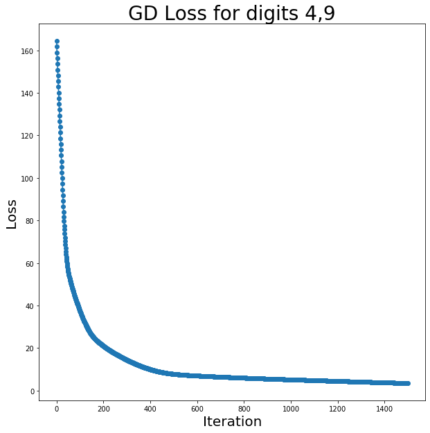
plotloss(gd_loss_list, title='GD Loss for digits 4,9', vis=None)
In [19]
train_accuracy, test_accuracy = classify(gd_weights, class_labels=[9, 4])
print('The accuracy rate for the training data is: ', train_accuracy)
print('The accuracy rate for the test data is: ', test_accuracy)
The accuracy rate for the training data is:  0.981
The accuracy rate for the test data is:  0.925
The accuracy for 4, 9 was fairly high. Now let's try 0,1.
In [20]
train_sample = process_data(train,
                            class_labels=[0, 1],
                            num_samples=500,
                            method=None)
tic = time()
v = np.ones(train_sample.shape[1] - 1)
gd_loss_list01, gd_weights01 = GD(w_init=v,
                                  learning_rate=10e-2,
                                  X=train_sample,
                                  tol=10e-6)
toc = time()
print(f" Gradient Descent runtime: {toc-tic:.2f} seconds.")
Gradient Descent runtime: 47.95 seconds.
In [21]
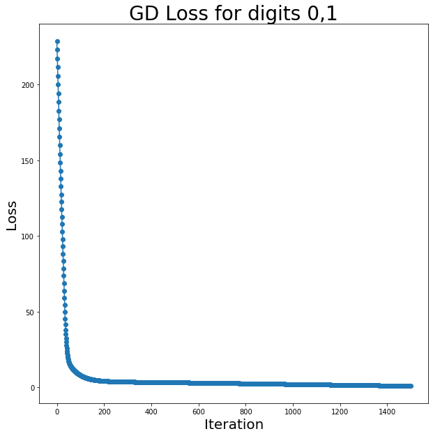
plotloss(gd_loss_list01, title='GD Loss for digits 0,1')
In [22]
train_accuracy, test_accuracy = classify(gd_weights01, class_labels=[0, 1])
print('The accuracy rate for the training data is: ', train_accuracy)
print('The accuracy rate for the test data is: ', test_accuracy)
The accuracy rate for the training data is:  0.998
The accuracy rate for the test data is:  0.995
The accuracy for 0,1 is higher. This makes sense because 0,1 are very dissimilar in terms of pixel overlap, whereas 4 and 9 have a bit more overlap, so we can expect less accuracy comparing those digits. Now let's compare 3 and 8, another set of fairly similar-looking digits.
In [23]
train_sample = process_data(train,
                            class_labels=[3, 8],
                            num_samples=500,
                            method=None)
tic = time()
v = np.ones(train_sample.shape[1] - 1)
gd_loss_list38, gd_weights38 = GD(w_init=v,
                                  learning_rate=10e-2,
                                  X=train_sample,
                                  tol=10e-6)
toc = time()
print(f" Gradient Descent runtime: {toc-tic:.2f} seconds.")
Gradient Descent runtime: 46.57 seconds.
In [24]
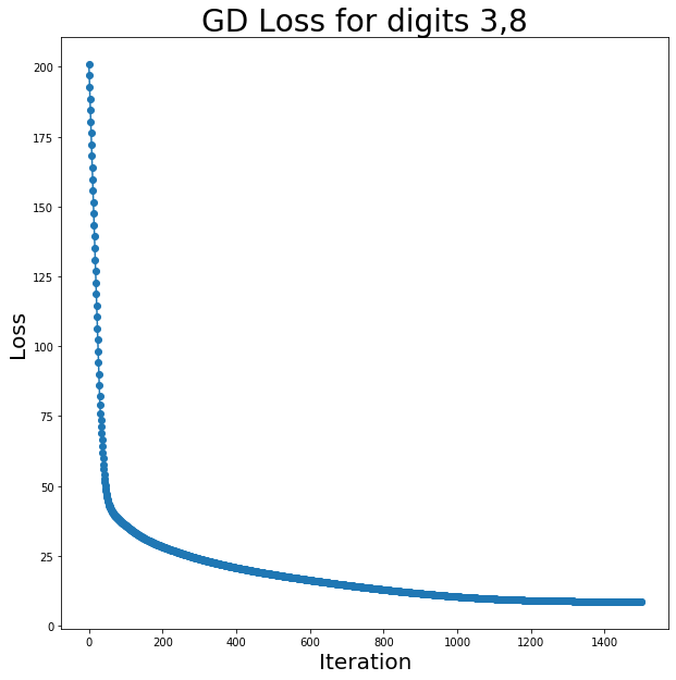
plotloss(gd_loss_list38, title='GD Loss for digits 3,8')
In [25]
train_accuracy, test_accuracy = classify(gd_weights38, class_labels=[3, 8])
print('The accuracy rate for the training data is: ', train_accuracy)
print('The accuracy rate for the test data is: ', test_accuracy)
The accuracy rate for the training data is:  0.972
The accuracy rate for the test data is:  0.919
Note the accuracy is a bit lower for these digits, as expected.
Gradient descent with momentum
Gradient descent with momentum, or Polyak momentum, is an improvement upon GD that uses the same basic idea of the GD, but gets a little more precise by incentivizing the algorithm to move further in the direction of the negative gradient if the previous iterate was also moving in that direction, and take shorter steps in the wrong direction (ie where the loss increases) by penalizing those steps where the direction of the gradient and the previous step don't match. It does this by adding a "momentum" term, so the update steps look like: $$ w^{(t+1)} = w^{(t)} - \mu \nabla_{w}f + \beta (w^{t} - w^{t-1})$$
Here, $\beta$ is chosen in a similar manner to the learning rate $\mu$; in the demo, we will limit our methods to trial and error for $\beta$. However, a more
Gradient descent with classical momentum demo
We will use the following function for GD with momentum; this function is similar to the GD function we had, but we will include a momentum term to see how it compares to vanilla GD. Going forward we will only compare the digit sets [0,1] and [3,8] to focus on the impact in accuracy of the methodology on similar and dissimilar digits
In [26]
Code: 37 lines
def GD_momentum(w_init, learning_rate, beta, X, tol):
    '''

    This function performs the gradient descent with classical momentum update steps, with the stoppping criteria as before.

    Parameters: an initial weight vector w, a learning rate, a beta value for the momentum strength, a dataset X, a
    tolerance threshold for the gradient norm

    Output: a list of the loss values at each iterate and a trained weight vector w

    '''
    c = 0
    loss_vals = []
    m = learning_rate
    err = tol + 1
    w = w_init
    b = beta
    temp = w.copy()

    while (err > tol) and (c < 1500):

        p = gradient(w, X)

        if c > 0:
            w_prev = temp.copy()
            temp = w.copy()
            w += -p * m + b * (w - w_prev)

        else:
            w -= p * m

        h = loss(w, X)
        loss_vals.append(h)

        c += 1
        err = np.linalg.norm(p)
    return loss_vals, w
In [27]
train_sample = process_data(train,
                            class_labels=[0, 1],
                            num_samples=500,
                            method=None)
tic = time()
v = np.ones(train_sample.shape[1] - 1)
gdm_loss_list, gdm_weights = GD_momentum(w_init=v,
                                         learning_rate=10e-2,
                                         beta=0.9,
                                         X=train_sample,
                                         tol=10e-6)
toc = time()
print(f" GD with momentum runtime: {toc-tic:.2f} seconds.")
GD with momentum runtime: 46.94 seconds.
In [28]
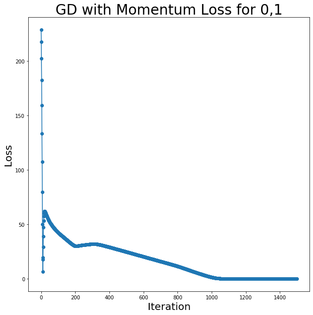
plotloss(gdm_loss_list, title='GD with Momentum Loss for 0,1')
In [29]
train_accuracy, test_accuracy = classify(gdm_weights, class_labels=[0, 1])
print('The accuracy rate for the training data is: ', train_accuracy)
print('The accuracy rate for the test data is: ', test_accuracy)
The accuracy rate for the training data is:  1.0
The accuracy rate for the test data is:  0.998
In [30]
train_sample = process_data(train,
                            class_labels=[4, 9],
                            num_samples=500,
                            method=None)
tic = time()
v = np.ones(train_sample.shape[1] - 1)
gdm_loss_list49, gdm_weights49 = GD_momentum(w_init=v,
                                             learning_rate=10e-2,
                                             beta=0.9,
                                             X=train_sample,
                                             tol=10e-6)
toc = time()
print(f" GD with momentum runtime: {toc-tic:.2f} seconds.")
GD with momentum runtime: 48.06 seconds.
In [31]
plotloss(gdm_loss_list49, title='GD with Momentum Loss for 4,9')
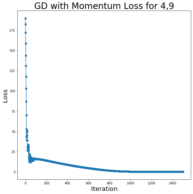
In [32]
train_accuracy, test_accuracy = classify(gdm_weights49, class_labels=[4, 9])
print('The accuracy rate for the training data is: ', train_accuracy)
print('The accuracy rate for the test data is: ', test_accuracy)
The accuracy rate for the training data is:  0.999
The accuracy rate for the test data is:  0.937
Note the accuracy on both the training and the test data is higher with momentum. We will now explore a variant of GD with momentum, called Nesterov's Acceleration Gradient (also called NAG). It is similar to GD with momentum, but it performs the algorithm in two update steps:
1. First, we take a step in the "momentum direction", the direction of the previous two steps.
2. Next, we take a gradient descent step from the momentum step, ie toward the direction of the negative gradient.
By doimg this, the algorithm includes a penalty term in the gradient as well if the previous two steps were not in the same direction (unlike momentum, which only included this penalty with the overall algorithm). In mathematical terms, we need to define a new variable $y^{(t)}$ and update as follows:
$$ y^{(t)} = w^{(t)} + \beta (w^{(t)} - w^{(t-1)})$$
$$ w^{(t+1)} = y^{(t)} - \mu \nabla f(y^{(t)})$$
We can combine these to get:
$$ w^{(t+1)} = w^{(t)} + \beta (w^{(t)} - w^{(t-1)}) - \mu \nabla f(w^{(t)} + \beta (w^{(t)} - w^{(t-1)}))$$
Nesterov's Accelerated Gradient demo
In [33]
Code: 34 lines
def NAG(w_init, learning_rate, beta, X, tol):
    '''

    This function performs the Nesterov's Accelerated Gradient update steps, with the stoppping criteria as described above.

    Parameters: an initial weight vector w, a learning rate,  a beta value for the momentum strength, a dataset X, a tolerance threshold for the gradient norm

    Output: a list of the loss values at each iterate and a trained weight vector w

    '''
    c = 0
    loss_vals = []
    m = learning_rate
    err = tol + 1
    w = w_init
    b = beta
    temp = w.copy()

    while (err > tol) and (c < 1500):
        if c > 0:
            w_prev = temp.copy()
            temp = w.copy()
            y = w + b * (w - w_prev)
            w = y - m * gradient(y, X)

        else:
            w -= m * gradient(w, X)

        h = loss(w, X)
        loss_vals.append(h)
        err = np.linalg.norm(h)

        c += 1
    return loss_vals, w
In [34]
train_sample = process_data(train,
                            class_labels=[0, 1],
                            num_samples=500,
                            method=None)
tic = time()
v = np.ones(train_sample.shape[1] - 1)
nag_loss_list, nag_weights = NAG(w_init=v,
                                 learning_rate=10e-2,
                                 beta=0.9,
                                 X=train_sample,
                                 tol=10e-6)
toc = time()
print(f" Nesterovs Accelerated Gradient runtime: {toc-tic:.2f} seconds.")
Nesterovs Accelerated Gradient runtime: 49.51 seconds.
In [35]
plotloss(nag_loss_list, title='Nesterovs Accelerated Gradient Loss for 0,1')
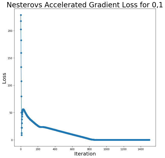
In [36]
train_accuracy, test_accuracy = classify(nag_weights, class_labels=[0, 1])
print('The accuracy rate for the training data is: ', train_accuracy)
print('The accuracy rate for the test data is: ', test_accuracy)
The accuracy rate for the training data is:  1.0
The accuracy rate for the test data is:  0.998
Note the accuracy is the same as classical momentum for the digits 0,1. Let's see if we see a difference in similar-looking digits like 4 and 9.
In [37]
train_sample = process_data(train,
                            class_labels=[4, 9],
                            num_samples=500,
                            method=None)
tic = time()
v = np.ones(train_sample.shape[1] - 1)
nag_loss_list49, nag_weights49 = NAG(w_init=v,
                                     learning_rate=10e-2,
                                     beta=0.9,
                                     X=train_sample,
                                     tol=10e-6)
toc = time()
print(f" Nesterovs Accelerated Gradient runtime: {toc-tic:.2f} seconds.")
Nesterovs Accelerated Gradient runtime: 48.67 seconds.
In [38]
plotloss(nag_loss_list49, title='Nesterovs Accelerated Gradient Loss for 4,9')
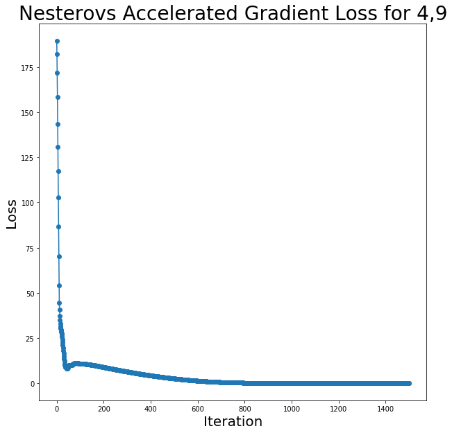
In [39]
train_accuracy, test_accuracy = classify(nag_weights49, class_labels=[4, 9])
print('The accuracy rate for the training data is: ', train_accuracy)
print('The accuracy rate for the test data is: ', test_accuracy)
The accuracy rate for the training data is:  0.999
The accuracy rate for the test data is:  0.939
Note the accuacy is higher with NAG than classical momentum for digits 4,9, but the improvement is very slight, which makes sense since our learning rate is small. With a larger sample size or more iterations, we might see some more distict differences in accuracy.
Conjugate Gradient Descent
Conjugate gradient descent is yet another variant of GD that uses conjugacy in order to converge more quickly and accurately. Conjugacy occurs when a set of vectors ${P_{1}, P_{2}, ..., P_{k}}$ and a symmetric positive definate matrix $A$ are such that ${P_{i}}^T A P_{j} = 0$ for all $i,j$ where $i \neq j$. We can minimize the loss by successively minimizing it along individual directions in a conjugate set. The conjugate direction method does this by using a predefined conjugate set of vectors ${P_{1}, P_{2}, ..., P_{k}}$, and updating weights like so:
$$ w^{(t+1)} = w^{(t)} + \alpha_{t} P_{t} $$
$$ \alpha_{t} = argmax_{a \in R} F(w^{t} + aP_{t})$$
Short detour into backtracking line search:
We would like to solve for $\alpha_{t} $ using something like exact line search. Exact line search, also called backtracking line search, is a method of computing the learning rate at every iterate to make sure that it really is moving in a descent direction. To do this, we need to check if Armijo conditions are met, and if they are not, we need to make the learning rate smaller by some factor. It can be shown that if the learning rate meets the Armijo criteria, we can be sure we are moving to an descent direction more accurately (instead of overstepping or moving too slowly towards a local loss minimum). We claim a learning rate meets the Armijo condition if the following holds:
$$ F(w - \mu \nabla F(w)) \leq F(w) - c_{1} \mu || \nabla F(w)||^{2}$$
Note we fix $c_{1} \in [0,1/2)$ in this definition. This condition, along with the following condition, make up a set of conditions called Wolfe's conditions:
$$|\nabla F(w^{(t)} + \alpha_{t}P_{t})^{T}P_{t}| \leq -c_{2} \nabla F_{t}^{T}P_{t}$$
Here we pick $c_{2} \in [c_{1},\frac{1}{2}]$. We will use Wolfe's conditions for the demo of CGD.
Back to conjugate methods:
This summarizes the conjugate direction method. However, we can improve upon this by using conjugate gradient method in order to avoid storing an extra set of conjugate vectors (${P_{1}, P_{2}, ..., P_{k}}$) by computing a vector at each iteration that is conjugate to all the previous vectors. We can do this by setting $$P_{t} = -\nabla F(w^{(t)}) + \beta_{t} P_{t-1}$$ We also need to iterate $\beta_{t}$ in order to enforce conjugacy. It can be shown that if we pick $$\beta_{t} = \frac{P_{t-1}^{T} A \nabla F(w^{(t)})}{P_{t-1}^{T} P_{t-1}} $$ where $A$ is the pixel matrix, we can enforce conjugacy. Other methods of updating $\beta$ that preserve conjugacy include the Fletcher-Reeves algorithm, which updates $\beta$ using the following equation: $$\beta_{t+1}^{F-R}= \frac{\nabla F_{t+1}^{T}\nabla F_{t+1}}{\nabla F_{t}^{T}\nabla F_{t}}$$ We can also use the Polak-Ribière update method, which updates $\beta$ via $$\beta_{t+1}^{P-R} = \frac{\nabla F_{t+1}^{T}(\nabla F_{t+1}^{T} - \nabla F_{t}^{T})}{|| \nabla F_{t})||^2}$$
In the demo below, we will explore the Fletcer-Reeves and Polak-Ribière variants of conjugate gradient descent for our dataset. Our update steps will be:
$$ w^{(t+1)} = w^{(t)} + \alpha_{t} P_{t} $$
<div align="center">
$ \alpha_{t}$ - update via backtracking line search
</div>
$$ \beta_{t+1}^{F-R}= \frac{\nabla F_{t+1}^{T}\nabla F_{t+1}}{\nabla F_{t}^{T}\nabla F_{t}} $$
<div align="center">
or
</div>
$$\beta_{t+1}^{P-R} = \frac{\nabla F_{t+1}^{T}(\nabla F_{t+1}^{T} - \nabla F_{t}^{T})}{|| \nabla F_{t})||^2}$$
$$ P_{t+1} = \nabla F_{t+1} + \beta_{t+1} P_{t} $$
Note we will need to define a new method for both backtacking line search and a check for the Wolfe criterion.
Conjugate Gradient Descent Demo
In [40]
def isWolfe(m, p, w, X):
    '''
    This method checks if the learning rate meets the Wolfe conditions.

    Parameters: a learning rate m, a conjugate vector p, the weight vector w, and the pixel data X

    Output: A True or False value of whether the
    '''
    c1 = 0.4
    c2 = 0.5
    if [
            loss((w + m * p), X) <=
            loss(w, X) + c1 * m * np.dot(gradient(w, X).T, p)
    ]:
        if [
                abs(np.dot(gradient(w + m * p, X), (X[:, 1:]).T / 255)) <=
                -c2 * np.dot(gradient(w, X), p)
        ]:
            return True
    else:
        return False
In [41]
def lineSearch(m, p, w, X):
    '''
    This method computes the learning rate via the backtracking line search, as outlined in the discussion.

    Parameters: a learning rate m, a conjugate vector p, a weight vector w, and the pixel data X

    Output: a scalar learning rate m
    '''
    while not isWolfe(m, p, w, X):
        m = 0.8 * m
    else:
        return m
In [42]
Code: 39 lines
def CGD(w_init, learning_rate, X, tol, method):
    '''

    This function performs the SGD update steps, with the stoppping criteria as before

    Parameters: an initial weight vector w, a learning rate, a dataset X, a tolerance threshold for the gradient norm

    Output: a list of the loss values at each iterate and a trained weight vector w

    '''
    if method not in ['F-R', 'P-R']:
        raise ValueError('Invalid method for CGD')

    c = 0
    loss_vals = []
    m = learning_rate
    err = tol + 1
    w = w_init
    new_grad = gradient(w, X)
    p = -new_grad

    while (c < 1500) and (err > tol):
        current_grad = new_grad.copy()
        m = lineSearch(m, p, w, X)
        w += m * p
        new_grad = gradient(w, X)
        if method == 'F-R':
            beta = np.dot(new_grad, new_grad) / np.dot(current_grad,
                                                       current_grad)
        else:
            if method == 'P-R':
                beta = np.dot(new_grad, new_grad - current_grad) / np.dot(
                    current_grad, current_grad)
        p = -new_grad + beta * p
        h = loss(w, X)
        loss_vals.append(h)
        err = np.linalg.norm(h)
        c += 1
    return loss_vals, w
In [43]
train_sample = process_data(train,
                            class_labels=[0, 1],
                            num_samples=500,
                            method=None)
tic = time()
v = np.ones(train_sample.shape[1] - 1)
cgd_loss_listFR, cgd_weightsFR = CGD(w_init=v,
                                     learning_rate=10e-2,
                                     X=train_sample,
                                     tol=10e-6,
                                     method='F-R')
toc = time()
print(
    f" Conjugate gradient descent with Fletcher-Reeves runtime: {toc-tic:.2f} seconds."
)
Conjugate gradient descent with Fletcher-Reeves runtime: 186.05 seconds.
In [44]
plotloss(cgd_loss_listFR,
         title='Conjugate Gradient Descent with Fletcher-Reeves Loss for 1,0')
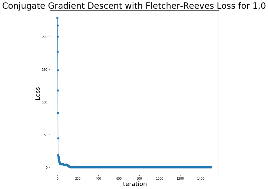
In [45]
train_accuracy, test_accuracy = classify(cgd_weightsFR, class_labels=[0, 1])
print('The accuracy rate for the training data is: ', train_accuracy)
print('The accuracy rate for the test data is: ', test_accuracy)
The accuracy rate for the training data is:  1.0
The accuracy rate for the test data is:  0.997
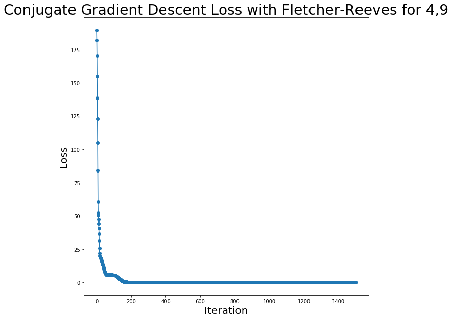
Clearly, this processs took a lot longer than other methods; this is expected due to the backtracking line search. We can also see we even lost a bit of accuracy with this method. Let's see if the same holds for 4,9.
In [46]
train_sample = process_data(train,
                            class_labels=[4, 9],
                            num_samples=500,
                            method=None)
tic = time()
v = np.ones(train_sample.shape[1] - 1)
cgd_loss_list49FR, cgd_weights49FR = CGD(w_init=v,
                                         learning_rate=10e-2,
                                         X=train_sample,
                                         tol=10e-6,
                                         method='F-R')
toc = time()
print(
    f" Conjugate gradient descent with Fletcher-Reeves runtime: {toc-tic:.2f} seconds."
)
Conjugate gradient descent with Fletcher-Reeves runtime: 185.34 seconds.
In [47]
plotloss(cgd_loss_list49FR,
         title='Conjugate Gradient Descent Loss with Fletcher-Reeves for 4,9')
In [48]
train_accuracy, test_accuracy = classify(cgd_weights49FR, class_labels=[4, 9])
print('The accuracy rate for the training data is: ', train_accuracy)
print('The accuracy rate for the test data is: ', test_accuracy)
The accuracy rate for the training data is:  1.0
The accuracy rate for the test data is:  0.931
In [49]
train_sample = process_data(train,
                            class_labels=[0, 1],
                            num_samples=500,
                            method=None)
tic = time()
v = np.ones(train_sample.shape[1] - 1)
cgd_loss_listPR, cgd_weightsPR = CGD(w_init=v,
                                     learning_rate=10e-2,
                                     X=train_sample,
                                     tol=10e-6,
                                     method='P-R')
toc = time()
print(
    f" Conjugate gradient descent with Polak-Ribière runtime: {toc-tic:.2f} seconds."
)
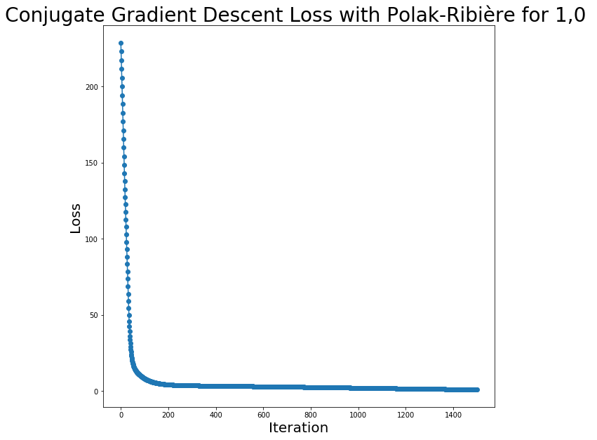
Conjugate gradient descent with Polak-Ribière runtime: 219.72 seconds.
In [50]
plotloss(cgd_loss_listPR,
         title='Conjugate Gradient Descent Loss with Polak-Ribière for 1,0 ')
In [51]
train_accuracy, test_accuracy = classify(cgd_weightsPR, class_labels=[0, 1])
print('The accuracy rate for the training data is: ', train_accuracy)
print('The accuracy rate for the test data is: ', test_accuracy)
The accuracy rate for the training data is:  0.998
The accuracy rate for the test data is:  0.995
In [52]
train_sample = process_data(train,
                            class_labels=[4, 9],
                            num_samples=500,
                            method=None)
tic = time()
v = np.ones(train_sample.shape[1] - 1)
cgd_loss_list49PR, cgd_weights49PR = CGD(w_init=v,
                                         learning_rate=10e-2,
                                         X=train_sample,
                                         tol=10e-6,
                                         method='P-R')
toc = time()
print(
    f" Conjugate gradient descent with Polak-Ribière runtime: {toc-tic:.2f} seconds."
)
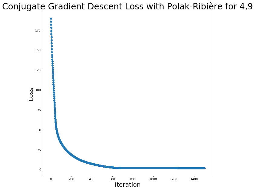
Conjugate gradient descent with Polak-Ribière runtime: 197.08 seconds.
In [53]
plotloss(cgd_loss_list49PR,
         title='Conjugate Gradient Descent Loss with Polak-Ribière for 4,9')
In [54]
train_accuracy, test_accuracy = classify(cgd_weights49PR, class_labels=[4, 9])
print('The accuracy rate for the training data is: ', train_accuracy)
print('The accuracy rate for the test data is: ', test_accuracy)
The accuracy rate for the training data is:  0.981
The accuracy rate for the test data is:  0.937
The accuracy has improved here in comparison to some previous methods. However, it is clear this method takes a long time to converge. We can modify that with stochastic gradient descent.
Stochastic Gradient Descent
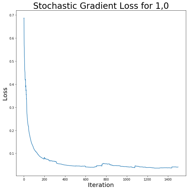
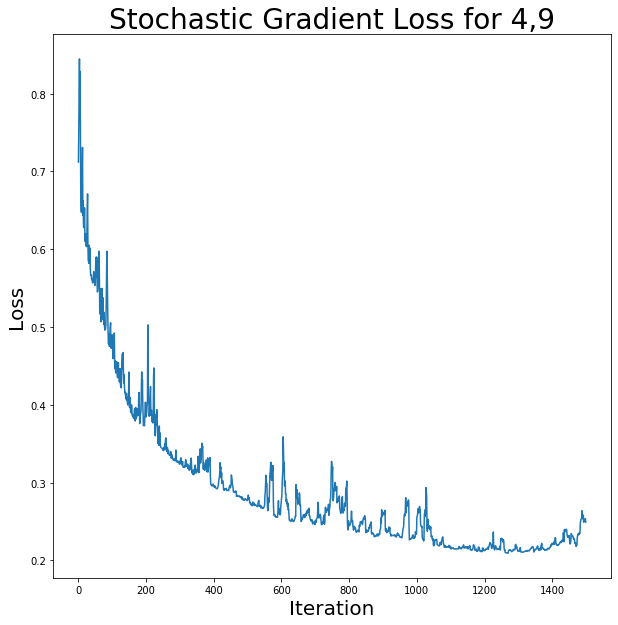
We've looked at various GD variants and gotten to a good accuracy using those methods. However, these have been pretty computationally expensive, so we should examine methods that are faster or converge sooner. One method that is computationally less expensive than vanilla GD is stochastic gradient descent, or SGD. GD and SGD share the same idea in that they both optimize using the direction of the negative gradient; in SGD however, we seek to make the gradient calculation (which happens at each iteration) faster, so instead of taking the gradient of all of the datapoints, we take the gradient of a single datapoint, sampled at random without replacement at each iterate. Our update step then looks like: $$ w^{(t+1)} = w^{(t)} - \mu \nabla_{w_{t}}f$$
where $\nabla_{w_{i_{t}}}f $ denotes the gradient of the loss function at iterate t with respect to some datapoint $x_{i_{t}}$ (here, $i_{t}$ is a random variable). This will allow for faster calculations of the gradient, since we only have to evaluate at one point; however, since the datapoints are chosen at random, we can expect to see more variance in the loss, as the datapoints might give different directions for the gradient. In the demo, we will redefine the function that performs the update step for the weights as well as the gradient calculation method. We'll also need to use a smaller learning rate in order to reduce the variance.
Stochastic Gradient Descent demo
In [55]
def stochastic_gradient(w, x_i):
    '''
    This method computes the gradient for SGD with respect to one randomly chosen datapoint.

    Parameters: a weight vector w, a randomly chosen datapoint x_i

    Output: a length 784 vector, the gradient of the loss at datapoint x_i
    '''
    y = x_i[0, 0]
    x_i = ((x_i[:, 1:]).T * y) / 225
    return (-x_i) / (1 + np.exp(np.dot(w.T, x_i)))
In [56]
def SGD(w_init, learning_rate, X, tol):
    '''

    This function performs the SGD update steps, with the stoppping criteria as before

    Parameters: an initial weight vector w, a learning rate, a dataset X, a tolerance threshold for the gradient norm

    Output: a list of the loss values at each iterate and a trained weight vector w

    '''
    c = 0
    loss_vals = []
    m = learning_rate
    err = tol + 1
    w = w_init
    N = X.shape[0]

    while (err > tol) and (c < 1500):
        random_index = np.random.choice(N, size=1, replace=True)
        dp_rand = X[random_index, :]
        p = stochastic_gradient(w, dp_rand)

        w -= m * p
        h = loss(w, X)
        loss_vals.append(h)
        err = np.linalg.norm(h)
        c += 1
    return loss_vals, w
In [57]
train_sample = process_data(train,
                            class_labels=[1, 0],
                            num_samples=500,
                            method=None)
tic = time()
v = np.zeros((train_sample.shape[1] - 1, 1))
sgd_loss_list, sgd_weights = SGD(w_init=v,
                                 learning_rate=10e-3,
                                 X=train_sample,
                                 tol=10e-6)
toc = time()
print(f" Stochastic Gradient Descent runtime: {toc-tic:.2f} seconds.")
Stochastic Gradient Descent runtime: 22.84 seconds.
In [58]
plotloss(sgd_loss_list, title='Stochastic Gradient Loss for 1,0', vis='smooth')
In [59]
train_accuracy, test_accuracy = classify(sgd_weights.T, class_labels=[1, 0])
print('The accuracy rate for the training data is: ', train_accuracy)
print('The accuracy rate for the test data is: ', test_accuracy)
The accuracy rate for the training data is:  0.999
The accuracy rate for the test data is:  1.0
In [60]
train_sample = process_data(train,
                            class_labels=[4, 9],
                            num_samples=500,
                            method=None)
tic = time()
v = np.zeros((train_sample.shape[1] - 1, 1))
sgd_loss_list49, sgd_weights49 = SGD(w_init=v,
                                     learning_rate=10e-3,
                                     X=train_sample,
                                     tol=10e-6)
toc = time()
print(f" Stochastic Gradient Descent runtime: {toc-tic:.2f} seconds.")
Stochastic Gradient Descent runtime: 21.03 seconds.
In [61]
plotloss(sgd_loss_list49,
         title='Stochastic Gradient Loss for 4,9',
         vis='smooth')
In [62]
train_accuracy, test_accuracy = classify(sgd_weights49.T, class_labels=[4, 9])
print('The accuracy rate for the training data is: ', train_accuracy)
print('The accuracy rate for the test data is: ', test_accuracy)
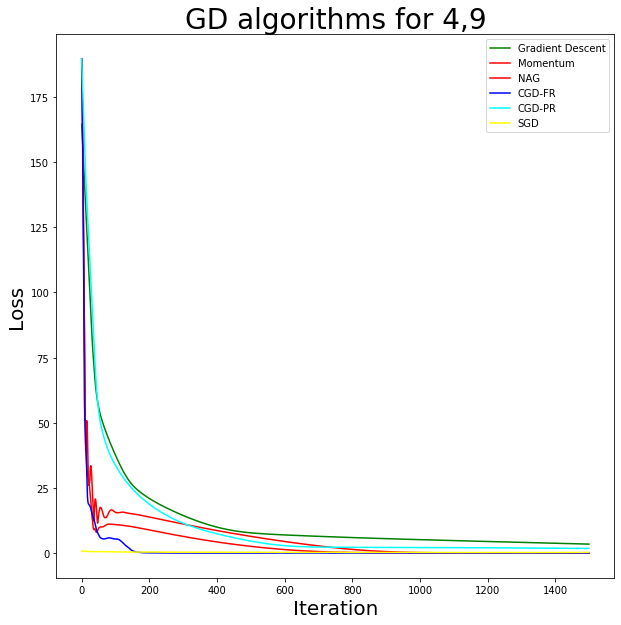
The accuracy rate for the training data is:  0.962
The accuracy rate for the test data is:  0.92
Visualizing each algorithm's performance
In [64]
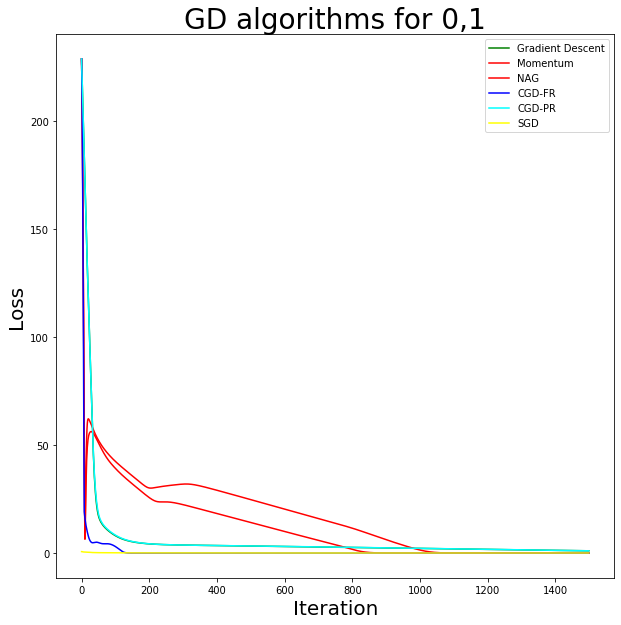
fig, ax = plt.subplots(1, 1, figsize=(10, 10))
ax.plot(gd_loss_list01, 'green', label = 'Gradient Descent')
ax.plot(gdm_loss_list, 'red', label = 'Momentum')
ax.plot(nag_loss_list, 'red', label = 'NAG')

ax.plot(cgd_loss_listFR, 'blue',label = 'CGD-FR')
ax.plot(cgd_loss_listPR, 'cyan', label = 'CGD-PR')
ax.plot(sgd_loss_list, 'yellow', label ='SGD')
ax.legend()
ax.set_xlabel("Iteration", fontsize=20)
ax.set_ylabel("Loss", fontsize=20)
ax.set_title('GD algorithms for 0,1', fontsize=28)
Text(0.5, 1.0, 'GD algorithms for 0,1')
In [65]
fig, ax = plt.subplots(1, 1, figsize=(10, 10))
ax.plot(gd_loss_list, 'green', label = 'Gradient Descent')
ax.plot(gdm_loss_list49, 'red', label = 'Momentum')
ax.plot(nag_loss_list49, 'red', label = 'NAG')

ax.plot(cgd_loss_list49FR, 'blue',label = 'CGD-FR')
ax.plot(cgd_loss_list49PR, 'cyan', label = 'CGD-PR')
ax.plot(sgd_loss_list49, 'yellow', label ='SGD')
ax.legend()
ax.set_xlabel("Iteration", fontsize=20)
ax.set_ylabel("Loss", fontsize=20)
ax.set_title('GD algorithms for 4,9', fontsize=28)
Text(0.5, 1.0, 'GD algorithms for 4,9')