Notebook · 2021
Tree Cover Prediction
Predicting Tree Type.ipynb
Notebook SHA-256 a2fcef05160d · 108 cells · 29 figures
Saved outputs shown as found. The notebook was not re-executed. 2 local path or credential pattern(s) were scrubbed before publication.
Forest Cover - Data Analysis and Prediction using Deep Learning
Introduction
In this project, we want to use a variety of algorithms and classifiers to predict the type of tree cover in a sample area within Roosevelt National Forest of Northern Colorado given various other features about the area, including the soil type, the vertical and horizontal distance to hydrology, the elevation, etc. We will use the following algorithms to make our predictions:
- K-Nearest Neighbor
- ExtraTrees
- Decision Trees
- Random Forest
- Light Gradient Boosting Machine
- XGBoost
We will do some data exploration, preprocessing, feature engineering, and other processes to ensure the algorithms we choose can make the best possible predictions.
Exploratory Data Analysis (EDA)
First, let's go through the exploratory stage of data analysis for this dataset, also called EDA. Here, we seek to understand the relationships between the features by creating graphs of their correlations, distributions, and skewness. Let's load some libraries we might use in this project.
In [55]
Code: 37 lines
# for data manipulation
import numpy as np
import pandas as pd
pd.set_option('display.max_columns', 60)
pd.set_option('display.max_rows', 60)

from IPython.display import display, HTML


# for visualization
from IPython.core.pylabtools import figsize
from matplotlib import pyplot as plt
%matplotlib inline
# to include graphs inline within the frontends next to code
import seaborn as sns
sns.set_context(font_scale=2)

# to bypass warnings in various dataframe assignments
pd.options.mode.chained_assignment = None

# machine learning models
from sklearn.neural_network import MLPClassifier

from sklearn.neighbors import KNeighborsClassifier
from sklearn.ensemble import RandomForestClassifier, ExtraTreesClassifier
from sklearn.tree import DecisionTreeClassifier
from xgboost import XGBClassifier
from lightgbm import LGBMClassifier

# preprocessing functions and evaluation models
from sklearn.model_selection import train_test_split
from sklearn.metrics import accuracy_score
from sklearn.dummy import DummyClassifier
from sklearn.preprocessing import StandardScaler
In [56]
trees = pd.read_csv("covtype.csv")
print("The size of the dataset is: ", trees.shape)
The size of the dataset is: (581012, 55)
This whole dataset has 581012 samples and 55 features. Let's look at the first 15 samples and the last 15 samples to see what some of this data looks like.
In [57]
display(HTML(trees.head(15).to_html()))
| Elevation | Aspect | Slope | Horizontal_Distance_To_Hydrology | Vertical_Distance_To_Hydrology | Horizontal_Distance_To_Roadways | Hillshade_9am | Hillshade_Noon | Hillshade_3pm | Horizontal_Distance_To_Fire_Points | Wilderness_Area1 | Wilderness_Area2 | Wilderness_Area3 | … | |
|---|---|---|---|---|---|---|---|---|---|---|---|---|---|---|
| 0 | 2596 | 51 | 3 | 258 | 0 | 510 | 221 | 232 | 148 | 6279 | 1 | 0 | 0 | … |
| 1 | 2590 | 56 | 2 | 212 | -6 | 390 | 220 | 235 | 151 | 6225 | 1 | 0 | 0 | … |
| 2 | 2804 | 139 | 9 | 268 | 65 | 3180 | 234 | 238 | 135 | 6121 | 1 | 0 | 0 | … |
| 3 | 2785 | 155 | 18 | 242 | 118 | 3090 | 238 | 238 | 122 | 6211 | 1 | 0 | 0 | … |
| 4 | 2595 | 45 | 2 | 153 | -1 | 391 | 220 | 234 | 150 | 6172 | 1 | 0 | 0 | … |
| 5 | 2579 | 132 | 6 | 300 | -15 | 67 | 230 | 237 | 140 | 6031 | 1 | 0 | 0 | … |
| 6 | 2606 | 45 | 7 | 270 | 5 | 633 | 222 | 225 | 138 | 6256 | 1 | 0 | 0 | … |
| 7 | 2605 | 49 | 4 | 234 | 7 | 573 | 222 | 230 | 144 | 6228 | 1 | 0 | 0 | … |
| 8 | 2617 | 45 | 9 | 240 | 56 | 666 | 223 | 221 | 133 | 6244 | 1 | 0 | 0 | … |
| 9 | 2612 | 59 | 10 | 247 | 11 | 636 | 228 | 219 | 124 | 6230 | 1 | 0 | 0 | … |
| 10 | 2612 | 201 | 4 | 180 | 51 | 735 | 218 | 243 | 161 | 6222 | 1 | 0 | 0 | … |
| 11 | 2886 | 151 | 11 | 371 | 26 | 5253 | 234 | 240 | 136 | 4051 | 1 | 0 | 0 | … |
Showing 12 of 15 rows and 14 of 56 columns. Full data is in the source notebook.
In [58]
display(HTML(trees.tail(15).to_html()))
| Elevation | Aspect | Slope | Horizontal_Distance_To_Hydrology | Vertical_Distance_To_Hydrology | Horizontal_Distance_To_Roadways | Hillshade_9am | Hillshade_Noon | Hillshade_3pm | Horizontal_Distance_To_Fire_Points | Wilderness_Area1 | Wilderness_Area2 | Wilderness_Area3 | … | |
|---|---|---|---|---|---|---|---|---|---|---|---|---|---|---|
| 580997 | 2433 | 168 | 23 | 162 | 41 | 175 | 231 | 241 | 128 | 815 | 0 | 0 | 1 | … |
| 580998 | 2429 | 166 | 24 | 153 | 45 | 162 | 232 | 240 | 125 | 812 | 0 | 0 | 1 | … |
| 580999 | 2426 | 168 | 24 | 150 | 42 | 153 | 231 | 241 | 127 | 811 | 0 | 0 | 1 | … |
| 581000 | 2423 | 169 | 24 | 134 | 39 | 150 | 230 | 241 | 128 | 810 | 0 | 0 | 1 | … |
| 581001 | 2421 | 172 | 25 | 124 | 35 | 134 | 227 | 242 | 132 | 811 | 0 | 0 | 1 | … |
| 581002 | 2419 | 168 | 25 | 108 | 33 | 124 | 230 | 240 | 126 | 812 | 0 | 0 | 1 | … |
| 581003 | 2415 | 161 | 25 | 95 | 29 | 120 | 236 | 237 | 116 | 815 | 0 | 0 | 1 | … |
| 581004 | 2410 | 158 | 24 | 90 | 24 | 120 | 238 | 236 | 115 | 819 | 0 | 0 | 1 | … |
| 581005 | 2405 | 159 | 22 | 90 | 19 | 120 | 237 | 238 | 119 | 824 | 0 | 0 | 1 | … |
| 581006 | 2401 | 157 | 21 | 90 | 15 | 120 | 238 | 238 | 119 | 830 | 0 | 0 | 1 | … |
| 581007 | 2396 | 153 | 20 | 85 | 17 | 108 | 240 | 237 | 118 | 837 | 0 | 0 | 1 | … |
| 581008 | 2391 | 152 | 19 | 67 | 12 | 95 | 240 | 237 | 119 | 845 | 0 | 0 | 1 | … |
Showing 12 of 15 rows and 14 of 56 columns. Full data is in the source notebook.
Here, we can see that the first 10 columns are continuous variables, describing some distance or angle, while the next 4 columns are one-hot encoded columns for the wilderness area of the sample. The winderness areas correspond with the following areas in the Roosevelt National Forest:
- Wilderness area 1 = Rawah Wilderness Area
- Wilderness area 2 = Neota Wilderness Area
- Wilderness area 3 = Comanche Peak Wilderness Area
- Wilderness area 4 = Cache la Poudre Wilderness Area
After the wilderness area columns, we have again one-hot encoded columns for 40 soil types, depending on what sort of soil the specific sample contains. The last column here is the cover type. This is a discrete variable with values 1-7 depending on the cover type. The numbers correspond with the following tree cover types:
- 1- Spruce/Fir
- 2- Lodgepole Pine
- 3- Ponderosa Pine
- 4- Cottonwood/Willow
- 5- Aspen
- 6- Douglas-fir
- 7- Krummholz
We should also look at the distribution of the values of each column to get a general sense of whether we need to consider any missing values, what the normal range for each feature looks like, and what they describe. The info and describe commands in from the pandas library can be useful for this.
In [59]
display(pd.DataFrame.info(trees))
print( 'Null values? :' , trees.isna().any().any())
Output: 63 lines
<class 'pandas.core.frame.DataFrame'>
RangeIndex: 581012 entries, 0 to 581011
Data columns (total 55 columns):
 #   Column                              Non-Null Count   Dtype
---  ------                              --------------   -----
 0   Elevation                           581012 non-null  int64
 1   Aspect                              581012 non-null  int64
 2   Slope                               581012 non-null  int64
 3   Horizontal_Distance_To_Hydrology    581012 non-null  int64
 4   Vertical_Distance_To_Hydrology      581012 non-null  int64
 5   Horizontal_Distance_To_Roadways     581012 non-null  int64
 6   Hillshade_9am                       581012 non-null  int64
 7   Hillshade_Noon                      581012 non-null  int64
 8   Hillshade_3pm                       581012 non-null  int64
 9   Horizontal_Distance_To_Fire_Points  581012 non-null  int64
 10  Wilderness_Area1                    581012 non-null  int64
 11  Wilderness_Area2                    581012 non-null  int64
 12  Wilderness_Area3                    581012 non-null  int64
 13  Wilderness_Area4                    581012 non-null  int64
 14  Soil_Type1                          581012 non-null  int64
 15  Soil_Type2                          581012 non-null  int64
 16  Soil_Type3                          581012 non-null  int64
 17  Soil_Type4                          581012 non-null  int64
 18  Soil_Type5                          581012 non-null  int64
 19  Soil_Type6                          581012 non-null  int64
 20  Soil_Type7                          581012 non-null  int64
 21  Soil_Type8                          581012 non-null  int64
 22  Soil_Type9                          581012 non-null  int64
 23  Soil_Type10                         581012 non-null  int64
 24  Soil_Type11                         581012 non-null  int64
 25  Soil_Type12                         581012 non-null  int64
 26  Soil_Type13                         581012 non-null  int64
 27  Soil_Type14                         581012 non-null  int64
 28  Soil_Type15                         581012 non-null  int64
 29  Soil_Type16                         581012 non-null  int64
 30  Soil_Type17                         581012 non-null  int64
 31  Soil_Type18                         581012 non-null  int64
 32  Soil_Type19                         581012 non-null  int64
 33  Soil_Type20                         581012 non-null  int64
 34  Soil_Type21                         581012 non-null  int64
 35  Soil_Type22                         581012 non-null  int64
 36  Soil_Type23                         581012 non-null  int64
 37  Soil_Type24                         581012 non-null  int64
 38  Soil_Type25                         581012 non-null  int64
 39  Soil_Type26                         581012 non-null  int64
 40  Soil_Type27                         581012 non-null  int64
 41  Soil_Type28                         581012 non-null  int64
 42  Soil_Type29                         581012 non-null  int64
 43  Soil_Type30                         581012 non-null  int64
 44  Soil_Type31                         581012 non-null  int64
 45  Soil_Type32                         581012 non-null  int64
 46  Soil_Type33                         581012 non-null  int64
 47  Soil_Type34                         581012 non-null  int64
 48  Soil_Type35                         581012 non-null  int64
 49  Soil_Type36                         581012 non-null  int64
 50  Soil_Type37                         581012 non-null  int64
 51  Soil_Type38                         581012 non-null  int64
 52  Soil_Type39                         581012 non-null  int64
 53  Soil_Type40                         581012 non-null  int64
 54  Cover_Type                          581012 non-null  int64
dtypes: int64(55)
memory usage: 243.8 MB
None
Null values? : False
Here, we can see all of the columns have non-null values and that the datatype for each is int64. The describe function will tell us more about the numerical distribution of each of these columns (or features).
In [60]
display(trees.describe())
| Elevation | Aspect | Slope | Horizontal_Distance_To_Hydrology | Vertical_Distance_To_Hydrology | Horizontal_Distance_To_Roadways | Hillshade_9am | Hillshade_Noon | Hillshade_3pm | Horizontal_Distance_To_Fire_Points | Wilderness_Area1 | Wilderness_Area2 | Wilderness_Area3 | … | |
|---|---|---|---|---|---|---|---|---|---|---|---|---|---|---|
| count | 581012.000000 | 581012.000000 | 581012.000000 | 581012.000000 | 581012.000000 | 581012.000000 | 581012.000000 | 581012.000000 | 581012.000000 | 581012.000000 | 581012.000000 | 581012.000000 | 581012.000000 | … |
| mean | 2959.365301 | 155.656807 | 14.103704 | 269.428217 | 46.418855 | 2350.146611 | 212.146049 | 223.318716 | 142.528263 | 1980.291226 | 0.448865 | 0.051434 | 0.436074 | … |
| std | 279.984734 | 111.913721 | 7.488242 | 212.549356 | 58.295232 | 1559.254870 | 26.769889 | 19.768697 | 38.274529 | 1324.195210 | 0.497379 | 0.220882 | 0.495897 | … |
| min | 1859.000000 | 0.000000 | 0.000000 | 0.000000 | -173.000000 | 0.000000 | 0.000000 | 0.000000 | 0.000000 | 0.000000 | 0.000000 | 0.000000 | 0.000000 | … |
| 25% | 2809.000000 | 58.000000 | 9.000000 | 108.000000 | 7.000000 | 1106.000000 | 198.000000 | 213.000000 | 119.000000 | 1024.000000 | 0.000000 | 0.000000 | 0.000000 | … |
| 50% | 2996.000000 | 127.000000 | 13.000000 | 218.000000 | 30.000000 | 1997.000000 | 218.000000 | 226.000000 | 143.000000 | 1710.000000 | 0.000000 | 0.000000 | 0.000000 | … |
| 75% | 3163.000000 | 260.000000 | 18.000000 | 384.000000 | 69.000000 | 3328.000000 | 231.000000 | 237.000000 | 168.000000 | 2550.000000 | 1.000000 | 0.000000 | 1.000000 | … |
| max | 3858.000000 | 360.000000 | 66.000000 | 1397.000000 | 601.000000 | 7117.000000 | 254.000000 | 254.000000 | 254.000000 | 7173.000000 | 1.000000 | 1.000000 | 1.000000 | … |
Showing 14 of 56 columns. Full data is in the source notebook.
Outlier Detection & Removal
We can see the ranges and the average value for each function. What we can't see so far is the distribution, so we don't know whether any outliers exist and if they create any problems in our analysis. To see this, we'll define a function to detect outliers in the dataset, using the inter quartile range (IQR) method. In this method, we calculate the first quarentile, Q1 and the third quarentile, Q3, and call the IQR the difference between the two. The IQR will then help us construct a normal range for the dataset using the following equations: $$UL = Q3 + 3\cdot IQR $$ $$LL = Q1 - 3\cdot IQR $$
Here, UL is the upper limit and LL is the lower limit. Values outside of this range will be considered outliers. Typically, 1.5 is used instead of 3 for ourliers, but I personally feel this excludes many samples that might be relevant. 3 is used to determine extreme outliers, so in order to keep our models flexible and accurate, we want to preserve as many rows as possible. This analysis mostly applies to continuous variables, so we will focus on the first 10 columns in selecting which outliers to exclude. We will also not consider the hillshade columns in this, as they have a pre-set range of 0-255, which does not require normalization.
In [61]
def find_outlier_IQR(df, col_name):
    '''
    This function takes in a dataset and a column name, and creates a normal range based on the IQR, and gives an outlier count.

    Parameters: a pandas dataframe, a string of column name in the dataframe

    Output: lower limit int , upper limit int, outlier count int

    '''
    Q1=np.percentile(np.array(df[col_name].tolist()), 25)
    Q3=np.percentile(np.array(df[col_name].tolist()), 75)
    IQR=Q3-Q1
    UL= Q3 + (3*IQR)
    LL= Q1 - (3*IQR)
    outlier_count = 0

    for value in df[col_name].tolist():
        if (value < LL) | (value > UL):
            outlier_count +=1

    return LL, UL, outlier_count


for column in trees[['Elevation', 'Aspect', 'Slope', 'Horizontal_Distance_To_Hydrology', 'Vertical_Distance_To_Hydrology', 'Horizontal_Distance_To_Roadways', 'Horizontal_Distance_To_Fire_Points']]:
    a,b,c =find_outlier_IQR(trees, column)
    if c > 0:
        print("There are {} outliers in {}. The normal range is {} - {}. ".format(c, column, a, b))
There are 275 outliers in Slope. The normal range is -18.0 - 45.0.
There are 414 outliers in Horizontal_Distance_To_Hydrology. The normal range is -720.0 - 1212.0.
There are 5339 outliers in Vertical_Distance_To_Hydrology. The normal range is -179.0 - 255.0.
There are 10 outliers in Horizontal_Distance_To_Fire_Points. The normal range is -3554.0 - 7128.0.
For this dataset, we will consider outliers from the following columns:
- Horizontal_Distance_To_Hydrology
- Vertical_Distance_To_Hydrology
- Horizontal_Distance_To_Fire_Points
This is becausem, as discussed earlier, the other columns are discrete variables (ie, one-hot encoded columns like soil type, wilderness area, etc) or have a pre-set range that does not need normalization, like the hillshade columns. We will first remove outliers from the Horizontal_Distance_To_Hydrology and Vertical_Distance_To_Hydrology columns, as they seem to have a wide range and a good number of outliers.
In [62]
trees = trees[(trees['Horizontal_Distance_To_Hydrology'] > find_outlier_IQR(trees, 'Horizontal_Distance_To_Hydrology')[0]) &
                (trees['Horizontal_Distance_To_Hydrology'] < find_outlier_IQR(trees, 'Horizontal_Distance_To_Hydrology')[1])&
                (trees['Vertical_Distance_To_Hydrology'] > find_outlier_IQR(trees, 'Vertical_Distance_To_Hydrology')[0]) &
                (trees['Vertical_Distance_To_Hydrology'] < find_outlier_IQR(trees, 'Vertical_Distance_To_Hydrology')[1])]
print(trees.shape)
(575348, 55)
In [63]
for column in trees[['Horizontal_Distance_To_Hydrology', 'Vertical_Distance_To_Hydrology', 'Horizontal_Distance_To_Roadways', 'Horizontal_Distance_To_Fire_Points']]:
    a,b,c =find_outlier_IQR(trees, column)
    if c > 0:
        print("There are {} outliers in {}. The normal range is {} - {}. ".format(c, column, a, b))
There are 66 outliers in Horizontal_Distance_To_Hydrology. The normal range is -705.0 - 1192.0.
There are 693 outliers in Vertical_Distance_To_Hydrology. The normal range is -173.0 - 247.0.
There are 5 outliers in Horizontal_Distance_To_Fire_Points. The normal range is -3568.0 - 7142.0.
This seems to have trimmed away some of the more extreme outliers from this dataset. Note that the Vertical_Distance_To_Hydrology column still has many outliers because the IQR is recomputing the ranges based on the new data, so these are not true extreme outliers, and we don't need to worry about them.
Univariate Analysis
Now that we have a bit of description about our dataset, let's begin univariate analysis on this dataset. In this section, we will look at the skew and densities of the varaibles. First, we have to split up the dataframe to destinguish the different types of variables, like continuous vs discrete (in this case, one-hot encoded) variables. As we saw, the continuous variables are the first 10 variables, so we will group them into a continuous variables list. The wilderness is one category of the ont-hot encoded columns, so will split that into a seperate list, and same with the soil type. This will make visualization easier as we want to avoid comparing different types of variables to one another.
In [64]
cont_vars = trees.loc[:,'Elevation':'Horizontal_Distance_To_Fire_Points']
cont_vars_vis = cont_vars.copy()
cont_vars_vis['Cover_Type'] = trees['Cover_Type']
soiltype = trees.loc[:,'Soil_Type1':'Soil_Type40']
soiltype_vis = soiltype.copy()
soiltype_vis['Cover_Type'] = trees['Cover_Type']
wilderness = trees.loc[:,'Wilderness_Area1':'Wilderness_Area4']
wilderness_vis = wilderness.copy()
wilderness_vis['Cover_Type'] = trees['Cover_Type']
print(wilderness.shape)
print(soiltype.shape)
print(cont_vars.shape)
(575348, 4)
(575348, 40)
(575348, 10)
First, let's see the distribution of the class, ie the tree cover type. Since we want to see it as a percentage of all cover types, a pie chart can best help us visualize this.
In [65]
labels= '1- Spruce/Fir', '2- Lodgepole Pine', '3- Ponderosa Pine', '4- Cottonwood/Willow', '5- Aspen', '6- Douglas-fir', '7- Krummholz'

trees_dist = trees.groupby('Cover_Type').size()
fig1, ax1 = plt.subplots()
fig1.set_size_inches(15,10)
ax1.pie(trees_dist, labels=labels, autopct='%1.1f%%')
ax1.axis('equal')
plt.title('Percentages of Tree Cover Types',fontsize=20)
plt.show()
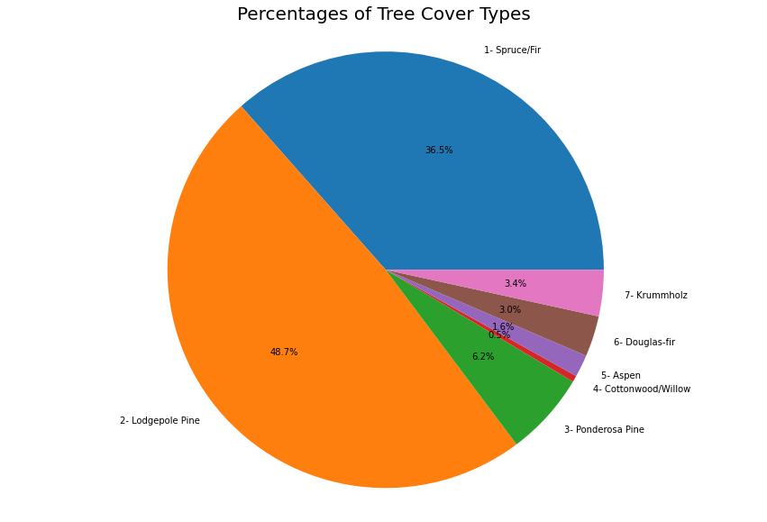
Clearly, the Lodgepole Pine and the Spruce/Fir are the most common types of trees in this sample.
Let's take a look at the skew to see if the outlier removal was able to mitigate the skew a bit. Recall skewness for a normal distribution is 0; this means the data is mostly even/symmentrical. Negative skew indicate that the column is "skewed left", which typically means the left tail, associated with relatively smaller values in the range, is longer than the right tail. Similarly, skewed right means the column has more relatively large values, which are in the right tail, and thus the right tail is longer than the left tail.
In [66]
skew = trees.skew()
display(skew)
Result: 56 lines
Elevation                              -0.841993
Aspect                                  0.408319
Slope                                   0.794381
Horizontal_Distance_To_Hydrology        1.067779
Vertical_Distance_To_Hydrology          1.259936
Horizontal_Distance_To_Roadways         0.711719
Hillshade_9am                          -1.179253
Hillshade_Noon                         -1.069709
Hillshade_3pm                          -0.286396
Horizontal_Distance_To_Fire_Points      1.284157
Wilderness_Area1                        0.194811
Wilderness_Area2                        4.039776
Wilderness_Area3                        0.272381
Wilderness_Area4                        3.561498
Soil_Type1                             13.673068
Soil_Type2                              8.579879
Soil_Type3                             10.785470
Soil_Type4                              6.610576
Soil_Type5                             18.901657
Soil_Type6                              9.207115
Soil_Type7                             74.003605
Soil_Type8                             56.667907
Soil_Type9                             22.329706
Soil_Type10                             3.843037
Soil_Type11                             6.594597
Soil_Type12                             4.032469
Soil_Type13                             5.573565
Soil_Type14                            30.943824
Soil_Type15                           437.927696
Soil_Type16                            14.115144
Soil_Type17                            12.850639
Soil_Type18                            17.319904
Soil_Type19                            11.836113
Soil_Type20                             7.691293
Soil_Type21                            26.145321
Soil_Type22                             3.781742
Soil_Type23                             2.660565
Soil_Type24                             4.934947
Soil_Type25                            34.796860
Soil_Type26                            14.806537
Soil_Type27                            26.897112
Soil_Type28                            27.351641
Soil_Type29                             1.501153
Soil_Type30                             4.026299
Soil_Type31                             4.454534
Soil_Type32                             2.860704
Soil_Type33                             3.195296
Soil_Type34                            18.985754
Soil_Type35                            17.356867
Soil_Type36                            69.511744
Soil_Type37                            43.905678
Soil_Type38                             5.836805
Soil_Type39                             6.242743
Soil_Type40                             8.560924
Cover_Type                              2.278729
dtype: float64
It seems the skewness is somewhat close to 0 for the continuous variables; let's visualize this to see what it looks like. This will help us get a better understanding of the skewnesss of variables relative to one another.
In [67]
skew =pd.DataFrame(skew,index=None,columns=['Skewness'])

plt.figure(figsize=(15,7))
sns.barplot(x=skew.index,y=skew.Skewness)
plt.xticks(rotation=90)
Result: 59 lines
(array([ 0,  1,  2,  3,  4,  5,  6,  7,  8,  9, 10, 11, 12, 13, 14, 15, 16,
        17, 18, 19, 20, 21, 22, 23, 24, 25, 26, 27, 28, 29, 30, 31, 32, 33,
        34, 35, 36, 37, 38, 39, 40, 41, 42, 43, 44, 45, 46, 47, 48, 49, 50,
        51, 52, 53, 54]),
 [Text(0, 0, 'Elevation'),
  Text(1, 0, 'Aspect'),
  Text(2, 0, 'Slope'),
  Text(3, 0, 'Horizontal_Distance_To_Hydrology'),
  Text(4, 0, 'Vertical_Distance_To_Hydrology'),
  Text(5, 0, 'Horizontal_Distance_To_Roadways'),
  Text(6, 0, 'Hillshade_9am'),
  Text(7, 0, 'Hillshade_Noon'),
  Text(8, 0, 'Hillshade_3pm'),
  Text(9, 0, 'Horizontal_Distance_To_Fire_Points'),
  Text(10, 0, 'Wilderness_Area1'),
  Text(11, 0, 'Wilderness_Area2'),
  Text(12, 0, 'Wilderness_Area3'),
  Text(13, 0, 'Wilderness_Area4'),
  Text(14, 0, 'Soil_Type1'),
  Text(15, 0, 'Soil_Type2'),
  Text(16, 0, 'Soil_Type3'),
  Text(17, 0, 'Soil_Type4'),
  Text(18, 0, 'Soil_Type5'),
  Text(19, 0, 'Soil_Type6'),
  Text(20, 0, 'Soil_Type7'),
  Text(21, 0, 'Soil_Type8'),
  Text(22, 0, 'Soil_Type9'),
  Text(23, 0, 'Soil_Type10'),
  Text(24, 0, 'Soil_Type11'),
  Text(25, 0, 'Soil_Type12'),
  Text(26, 0, 'Soil_Type13'),
  Text(27, 0, 'Soil_Type14'),
  Text(28, 0, 'Soil_Type15'),
  Text(29, 0, 'Soil_Type16'),
  Text(30, 0, 'Soil_Type17'),
  Text(31, 0, 'Soil_Type18'),
  Text(32, 0, 'Soil_Type19'),
  Text(33, 0, 'Soil_Type20'),
  Text(34, 0, 'Soil_Type21'),
  Text(35, 0, 'Soil_Type22'),
  Text(36, 0, 'Soil_Type23'),
  Text(37, 0, 'Soil_Type24'),
  Text(38, 0, 'Soil_Type25'),
  Text(39, 0, 'Soil_Type26'),
  Text(40, 0, 'Soil_Type27'),
  Text(41, 0, 'Soil_Type28'),
  Text(42, 0, 'Soil_Type29'),
  Text(43, 0, 'Soil_Type30'),
  Text(44, 0, 'Soil_Type31'),
  Text(45, 0, 'Soil_Type32'),
  Text(46, 0, 'Soil_Type33'),
  Text(47, 0, 'Soil_Type34'),
  Text(48, 0, 'Soil_Type35'),
  Text(49, 0, 'Soil_Type36'),
  Text(50, 0, 'Soil_Type37'),
  Text(51, 0, 'Soil_Type38'),
  Text(52, 0, 'Soil_Type39'),
  Text(53, 0, 'Soil_Type40'),
  Text(54, 0, 'Cover_Type')])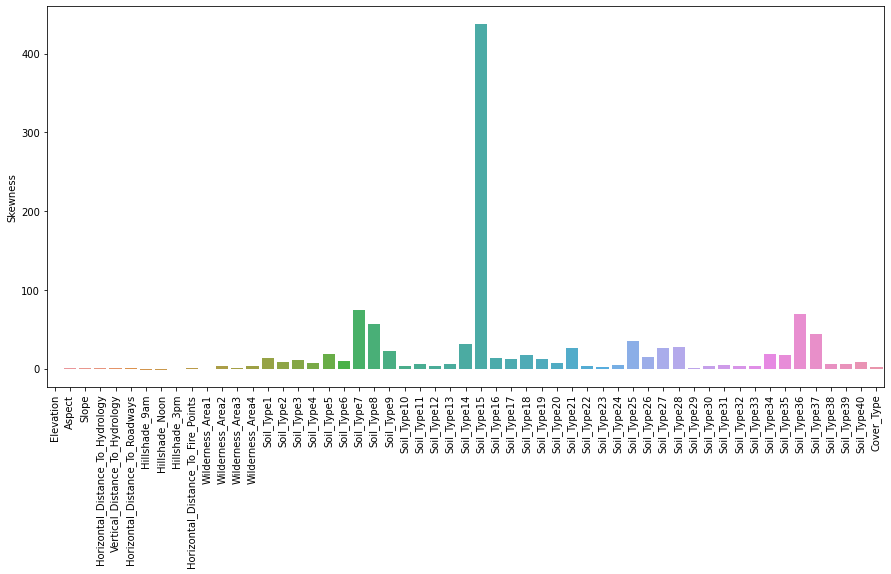
In [68]
plt.figure(figsize=(14, 28))
for i,col in enumerate(cont_vars.columns.values):
    l,u,ct = find_outlier_IQR(cont_vars_vis,col)
    plt.subplot(5,2,i+1)
    sns.kdeplot(cont_vars[col])
    plt.axvline(x=l, color = 'g')
    plt.axvline(x=u, color = 'r')

plt.show()
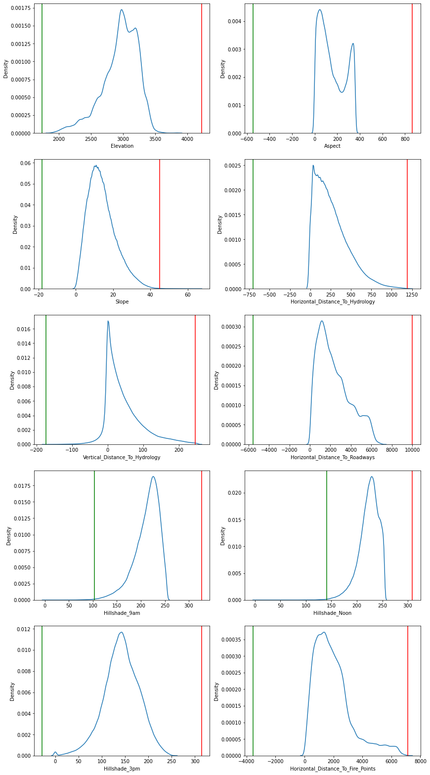
It seems our observations were correct, the most skewed features are the discrete or one-hot encoded features. This is probably not an issue since there is also a bias in the class representation (two types of trees are over-represented). We can see if we can explore some relationships between features during the bivariate and multivariate analysis.
Bivariate Analysis
Let's now begin the bivariate analysis phase. In bivariate analysis, we are looking at the relationship between features. First, we can look at the below boxplots to see each continuous variable's frequency with respect to the cover type.
In [69]
for i, col in enumerate(cont_vars.columns):
    plt.figure(i,figsize=(10,4))
    ax = sns.boxplot(x=cont_vars_vis['Cover_Type'], y=col, data=cont_vars_vis, palette="rocket")
    ax.set_xticklabels(labels, rotation=30)
    plt.show()
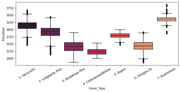
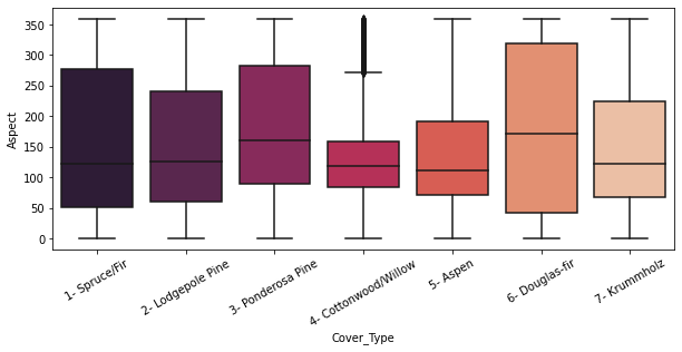
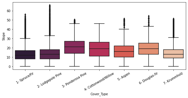
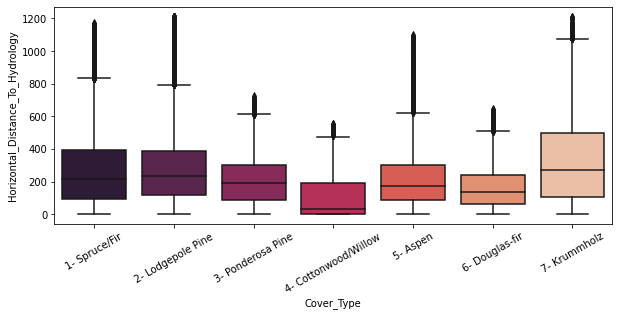
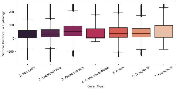
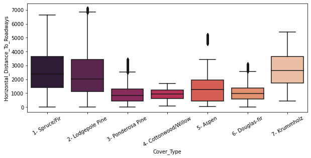
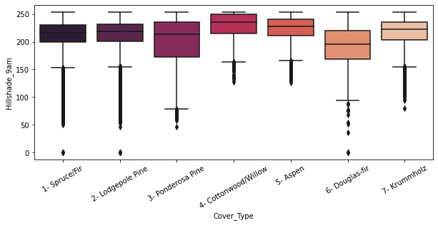
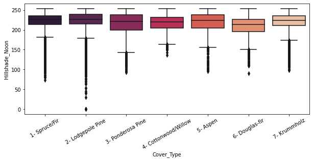
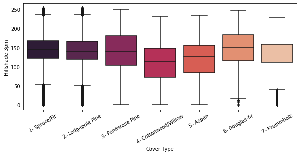
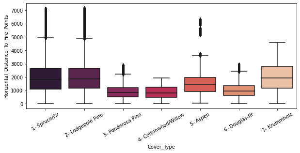
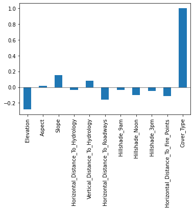
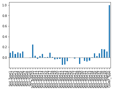
We can now take a look at the correlation of the variables to the cover type. First, lets see a summary; then, we can visualize these.
In [70]
corr = trees.corr()['Cover_Type']
corr = pd.DataFrame(data =corr)
corr = corr.rename({'Cover_Type': 'Correlation'}, axis = 1)
print(corr)
Output: 57 lines
                                    Correlation
Elevation                             -0.282160
Aspect                                 0.015804
Slope                                  0.152433
Horizontal_Distance_To_Hydrology      -0.032768
Vertical_Distance_To_Hydrology         0.079644
Horizontal_Distance_To_Roadways       -0.161764
Hillshade_9am                         -0.034286
Hillshade_Noon                        -0.098474
Hillshade_3pm                         -0.051531
Horizontal_Distance_To_Fire_Points    -0.113677
Wilderness_Area1                      -0.202592
Wilderness_Area2                      -0.047817
Wilderness_Area3                       0.063319
Wilderness_Area4                       0.327001
Soil_Type1                             0.091900
Soil_Type2                             0.119445
Soil_Type3                             0.068978
Soil_Type4                             0.099597
Soil_Type5                             0.078785
Soil_Type6                             0.114294
Soil_Type7                            -0.000464
Soil_Type8                            -0.003655
Soil_Type9                            -0.006050
Soil_Type10                            0.247147
Soil_Type11                            0.035921
Soil_Type12                           -0.023214
Soil_Type13                            0.025601
Soil_Type14                            0.066283
Soil_Type15                            0.006493
Soil_Type16                            0.010127
Soil_Type17                            0.091667
Soil_Type18                            0.007615
Soil_Type19                           -0.036583
Soil_Type20                           -0.028604
Soil_Type21                           -0.025545
Soil_Type22                           -0.142501
Soil_Type23                           -0.135571
Soil_Type24                           -0.068260
Soil_Type25                           -0.006435
Soil_Type26                           -0.000200
Soil_Type27                           -0.020906
Soil_Type28                           -0.001495
Soil_Type29                           -0.124597
Soil_Type30                           -0.009967
Soil_Type31                           -0.064387
Soil_Type32                           -0.075585
Soil_Type33                           -0.060780
Soil_Type34                            0.004903
Soil_Type35                            0.081246
Soil_Type36                            0.025681
Soil_Type37                            0.081109
Soil_Type38                            0.160906
Soil_Type39                            0.156542
Soil_Type40                            0.112593
Cover_Type                             1.000000
In [71]
ax = cont_vars_vis.corr()["Cover_Type"].plot(kind="bar")
ax.axhline(linewidth=0.5,y=0, color = 'k')
<matplotlib.lines.Line2D at 0x17e00d69df0>
In [72]
ax= soiltype_vis.corr()["Cover_Type"].plot(kind="bar")
ax.axhline(linewidth=0.5,y=0, color = 'k')
<matplotlib.lines.Line2D at 0x17e6014c7f0>
In [73]
ax = wilderness_vis.corr()["Cover_Type"].plot(kind="bar")
ax.axhline(linewidth=0.5,y=0, color = 'k')
<matplotlib.lines.Line2D at 0x17e6016dd00>
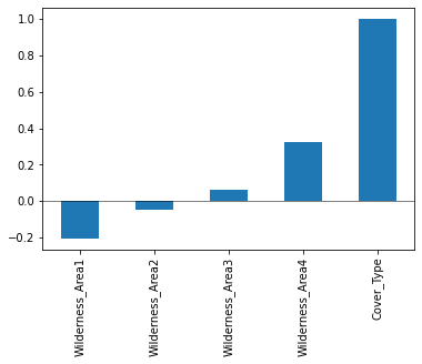
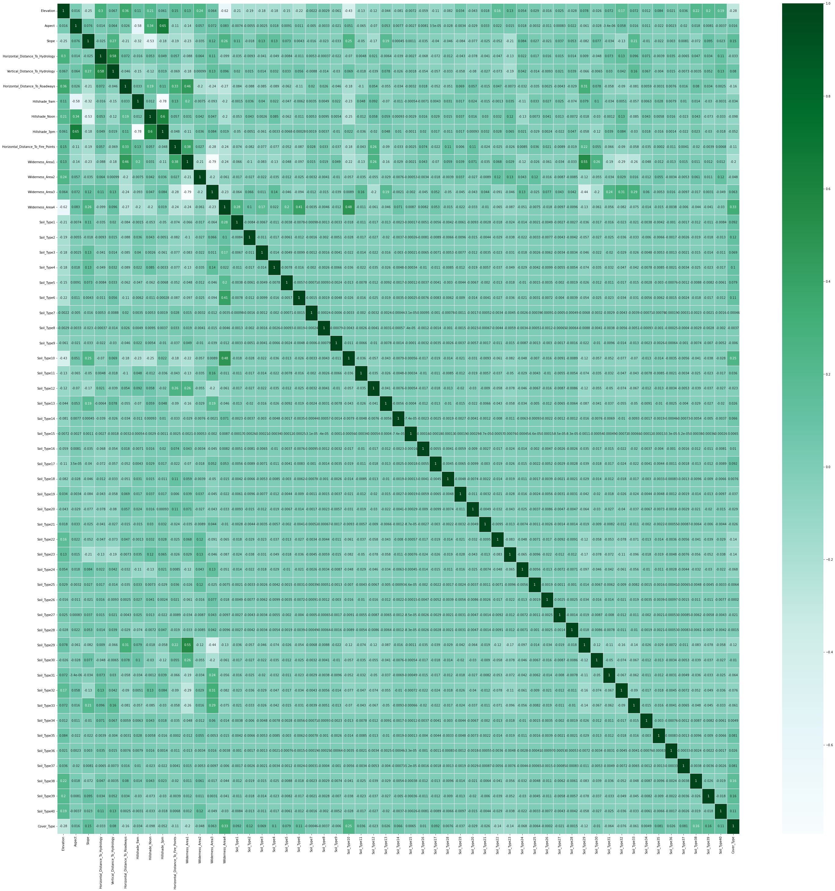
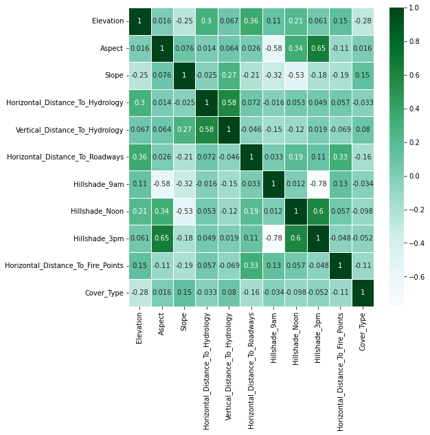
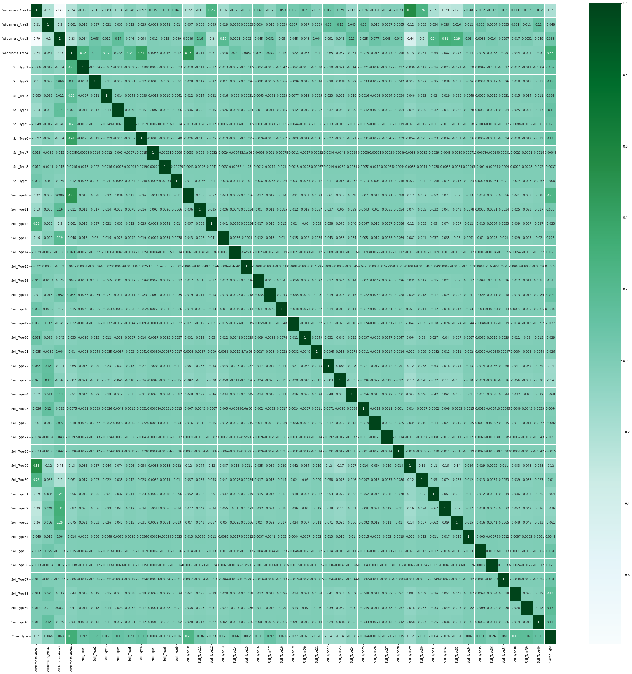
This tells us a lot about the correlation with respect to the class. We can also explore the correlation between every pair of features with the heat map of a correlation matrix below.
In [74]
plt.figure(figsize=(50,50))
sns.heatmap(trees.corr(),cmap='BuGn',linecolor='white',linewidths=1,annot=True, xticklabels = True, yticklabels= True)
<AxesSubplot:>
In [75]
plt.figure(figsize=(8,8))

sns.heatmap(cont_vars_vis.corr(),cmap='BuGn',linecolor='white',linewidths=1,annot=True, xticklabels = True, yticklabels= True)
<AxesSubplot:>
In [76]
plt.figure(figsize=(40,40))
disc = trees.drop(trees.columns[0:10], axis=1)
sns.heatmap(disc.corr(),cmap='BuGn',linecolor='white',linewidths=1,annot=True, xticklabels = True, yticklabels= True)
<AxesSubplot:>
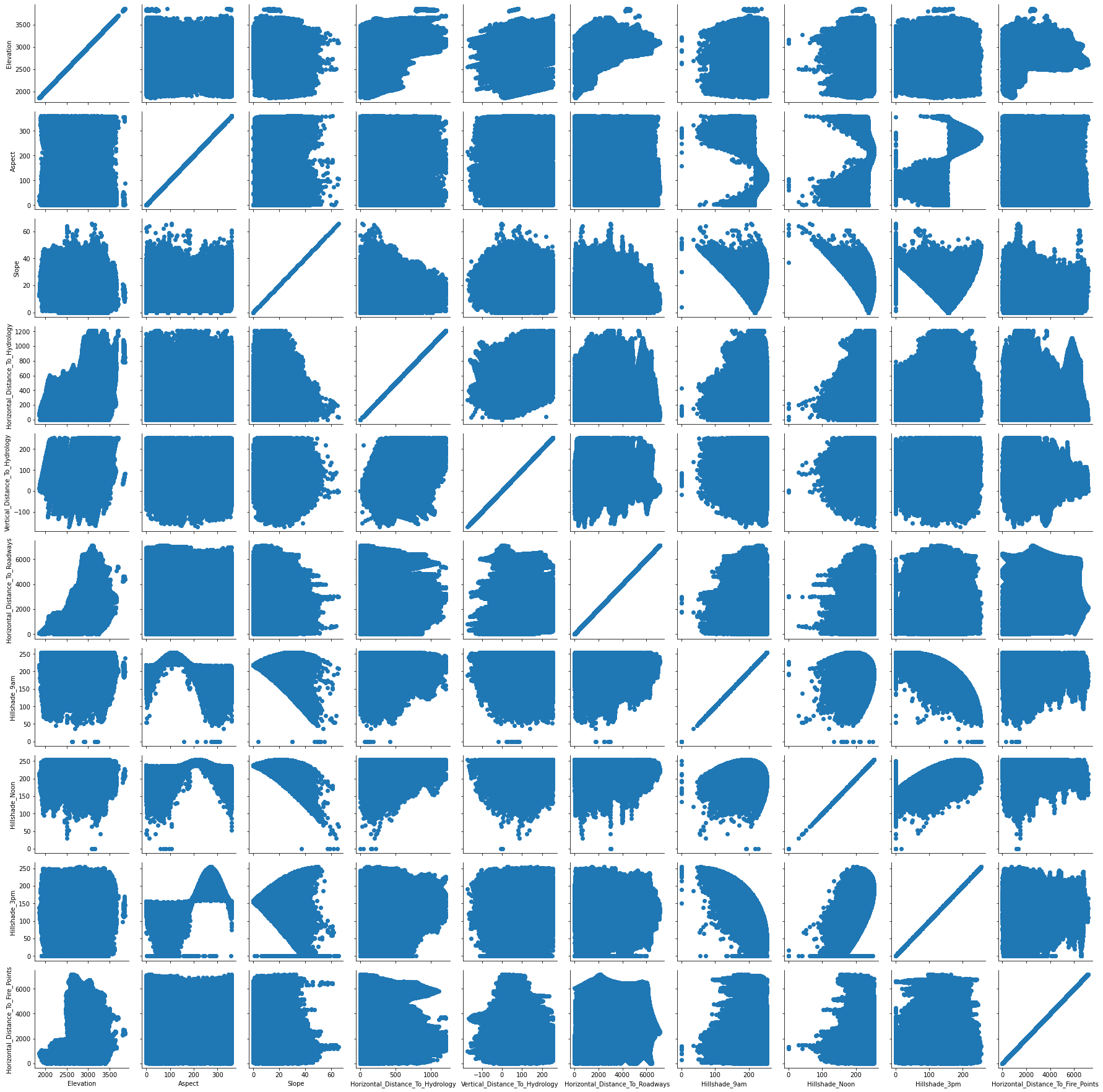
Let's visualize what some of these relationships between variables look like, at least with the continuous data.
In [77]
plt.figure(figsize=(8,8))

x = sns.PairGrid(cont_vars)
x.map(plt.scatter)
<seaborn.axisgrid.PairGrid at 0x17e2c723220>
<Figure size 576x576 with 0 Axes>
Conclusions from EDA
Our left-skewed variables are:
- Elevation
- Hillshade_9am
- Hillshade_Noon
- Hillshade_3pm
- Horizontal_Distance_To_Fire_Points
Our right-skewed variables are:
- Slope
- Horizontal_Distance_To_Roadways
The correlation offers some insight into the trends between variables. From the heat map, we can see the following positive and negative relationships:
Positive correlation pairs:
- Hillshade_9am and Aspect
- Hillshade_3pm and Aspect
- Horizontal_Distance_To_Hydrology and Vertical_Distance_To_Hydrology
- Horizontal_Distance_To_Roadways and Horizontal_Distance_To_Fire_Points
- Hillshade_3pm and Hillshade_Noon
Negative correlation pairs:
- Elevation and Horizontal_Distance_To_Hydrology
- Elevation and Horizontal_Distance_To_Roadways
- Aspect and Hillshade_9am
- Slope and Hillshade_Noon
- Hillshade_9am and Hillshade_3pm
- Wilderness_Area3 and Wilderness_Area1
Predicting trees with tree-based algorithms
We are finally ready to do some analysis on this dataset. Although we haven't done any sort of feature engineering to remove or add features yet, we will use tree-based algorithms to figure out some important features in the dataset. One helpful aspect of tree-based algorithms is that they do not require type c data preprocessing-- that is, normalization, feature selection/ dimensionality reduction, log transformation, etc. Thus, we can use this algorithm to simultaneously get started on our data analysis and get some insight into important features.
Establishing a Control Group
First, we will create a dummy algorithm to get a sort of control group for our later algorithms. This is also called a common-sense baseline, and it serves as a metric to make sure our algorithm is actually improving on an algorithm that follows minimal rules, as the DummyClassifier in scikit-learn does.
In [78]
acc =[]
algs = []
trees_training = trees.drop('Cover_Type', axis=1)
labels_training = trees["Cover_Type"]
train, test, train_labels, test_labels = train_test_split(trees_training, labels_training, test_size=0.3, random_state=1)
dummy = DummyClassifier(strategy='stratified', random_state=1)

# training the model with the training data (70% of our dataset)
dummy.fit(train, train_labels)

# get accuracy score, add it to our list for comparison later
baseline_accuracy = dummy.score(test, test_labels)
acc.append(baseline_accuracy)
algs.append('Dummy Classifier')
print("Our dummy algorithm classified {:0.2f}% of the of the trees correctly".format(baseline_accuracy*100))
Our dummy algorithm classified 37.65% of the of the trees correctly
So now we know we have to improve upon a 38% accuracy rate! I'm sure the decision trees and random forest algorithms can help with that.
Decision Tree
Since decision trees are one of the more basic tree-based algorithms, I wanted to see how it compared in this setting to random forests and ExtraTrees. Let's take a look at what the implementation of this looks like.
In [79]
dtree = DecisionTreeClassifier()
dtree.fit(train, train_labels)
dectree_pred = dtree.predict(test)
dtree_accuracy = accuracy_score(dectree_pred , test_labels)
acc.append(dtree_accuracy)
feat_dt = dtree.feature_importances_

algs.append('Decision Tree')
print("Our decision tree classified {:0.2f}% of the of the trees correctly".format(dtree_accuracy*100))
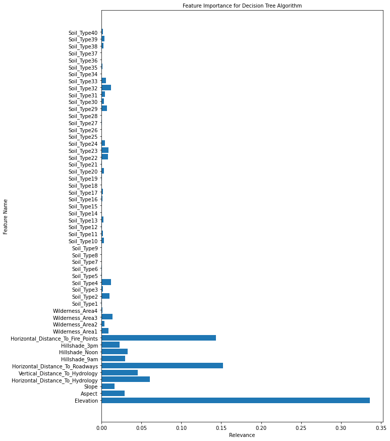
Our decision tree classified 93.55% of the of the trees correctly
Looks like the decision tree was pretty accurate! Let's take a look at what features this algorithm found important in prediction.
In [80]
plt.figure(figsize=(10,15))
plt.barh(train.columns.values, feat_dt)
plt.title('Feature Importance for Decision Tree Algorithm',fontsize=10)
plt.ylabel('Feature Name')
plt.xlabel('Relevance')
plt.show()
Random Forest
In [81]
rf = RandomForestClassifier()
rf.fit(train, train_labels)
rf_pred = rf.predict(test)
rf_acc = accuracy_score(rf_pred , test_labels)
acc.append(rf_acc)
algs.append('Random Forest')
feat_rf = rf.feature_importances_
print("Our random forest classified {:0.2f}% of the of the trees correctly".format(rf_acc*100))
Our random forest classified 95.22% of the of the trees correctly
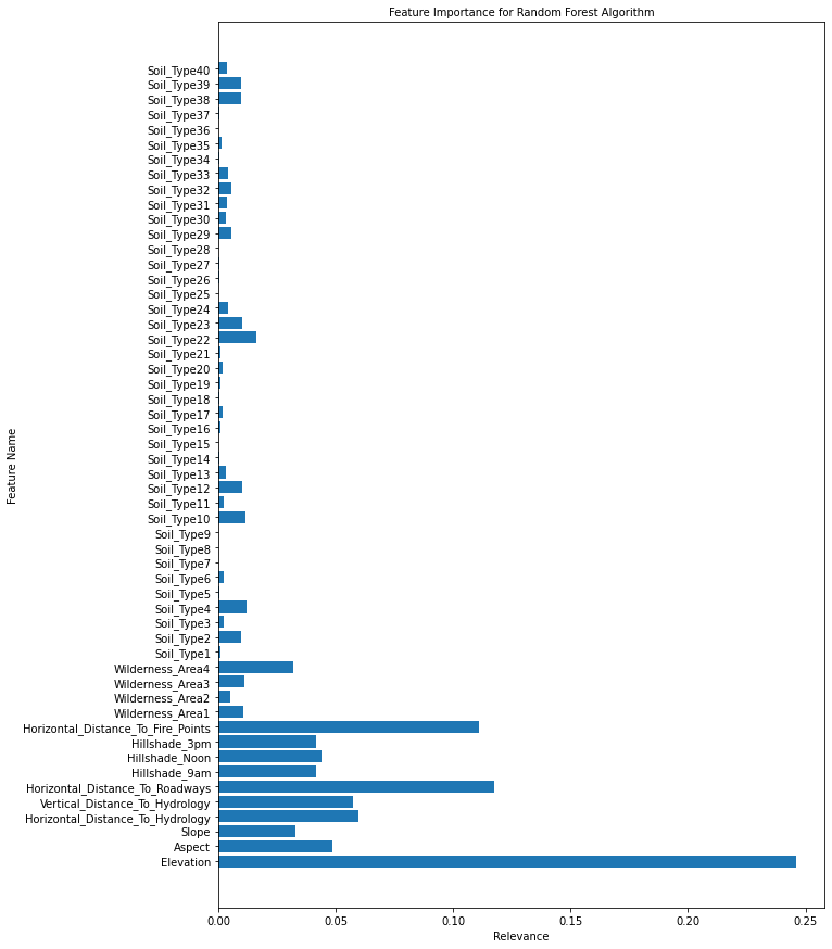
So we were able to obtain a 2% increase in accuracy! That's certainly quite an improvement, and although it took a lot longer than the decision tree. This is generally why many prefer random forests for accuracy, and why random forests are so popular in classification problems. Let's see if the feature importance is the same here.
In [82]
plt.figure(figsize=(10,15))
plt.barh(train.columns.values, feat_rf)
plt.title('Feature Importance for Random Forest Algorithm',fontsize=10)
plt.ylabel('Feature Name')
plt.xlabel('Relevance')
plt.show()
ExtraTrees
In [83]
etree = ExtraTreesClassifier()
etree.fit(train, train_labels)
etree_pred = etree.predict(test)
etree_acc = accuracy_score(etree_pred , test_labels)
acc.append(etree_acc)
algs.append('ExtraTrees')
feat_et = etree.feature_importances_
print("ExtraTrees classified {:0.2f}% of the of the trees correctly".format(etree_acc*100))
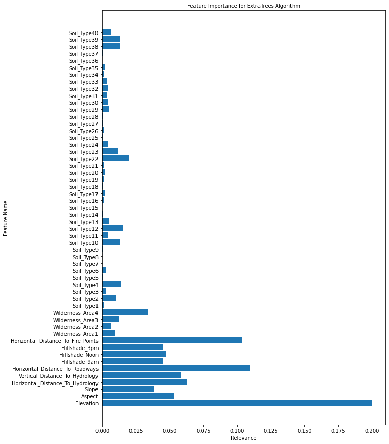
ExtraTrees classified 95.08% of the of the trees correctly
This algorithm actually performed somewhat on par with the random forest, although the random forest still beat it by a small margin.
In [84]
plt.figure(figsize=(10,15))
plt.barh(train.columns.values,feat_et)
plt.title('Feature Importance for ExtraTrees Algorithm',fontsize=10)
plt.ylabel('Feature Name')
plt.xlabel('Relevance')
plt.show()
Feature Selection
I have a feeling some soil types are under-represented. To investigate this, I will create a method that will turn soil type into a numerical value, or reverse-encode it. Then, we can create a pie chart to see which soil types are most common.
In [85]
def reverse_encode(relevant_subset):
    '''
    This function reverses one-hot encoding for into rank-encoded representations

    Parameters: an subset of relevant columns of the same type, which we are trying to reverse encode

    Output: a title-less list of the encoded variable in numerical data

    '''

    num_list =[]
    for i in relevant_subset.iloc:
        ix = 1
        for j in i:
            if j ==1:
                num_list.append(ix)
            else:
                ix +=1

    print('The new list has the following elements: ' + str(set(num_list)))
    if relevant_subset.shape[0] == len(num_list):
        return num_list
    else: print('Error in compiling list: lengths of the two lists do not match.')


w = reverse_encode(wilderness)
print(len(w))
The new list has the following elements: {1, 2, 3, 4}
575348
In [86]
s = reverse_encode(soiltype)
print(len(s))
The new list has the following elements: {1, 2, 3, 4, 5, 6, 7, 8, 9, 10, 11, 12, 13, 14, 15, 16, 17, 18, 19, 20, 21, 22, 23, 24, 25, 26, 27, 28, 29, 30, 31, 32, 33, 34, 35, 36, 37, 38, 39, 40}
575348
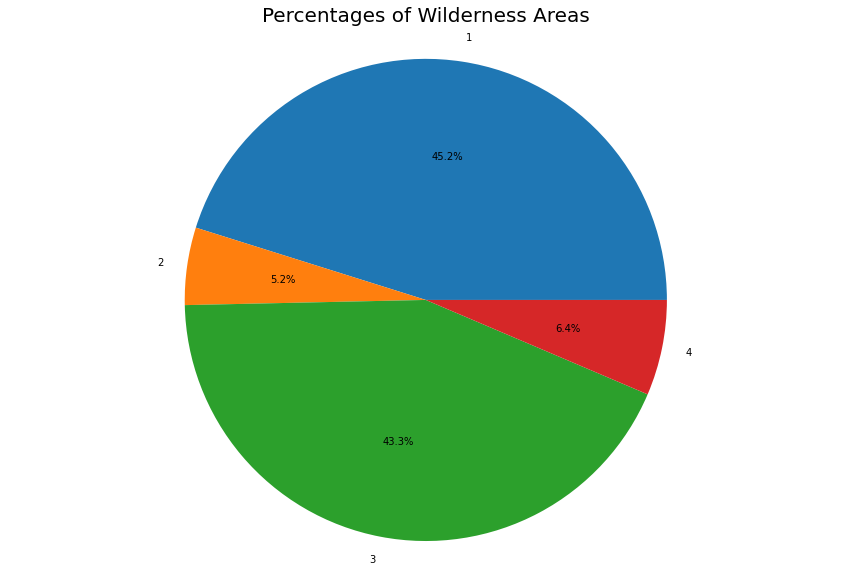
We were able to unencode the one-hot encoded variables successfully. Now let's see the plot chart for the wilderness area. Since soil type has more than 7 classes, its not as effective to visualize it with a pie chart. We can use a bar chart instead.
In [87]
lab =list(range(1,5))

w = pd.DataFrame(w, columns=['Wilderness'])
wild_dist = w.groupby('Wilderness').size()
fig1, ax1 = plt.subplots()
fig1.set_size_inches(15,10)
ax1.pie(wild_dist, labels= lab, autopct='%1.1f%%')
ax1.axis('equal')
plt.title('Percentages of Wilderness Areas',fontsize=20)
plt.show()
In [88]
s = pd.DataFrame(s,columns= ['Soil'] )
soil_dist = s.groupby('Soil').size()
print('Soil type with percentage of total')
print((soil_dist/sum(soil_dist))*100)
Output: 44 lines
Soil type with percentage of total
Soil
1      0.526464
2      1.305471
3      0.838101
4      2.142356
5      0.277571
6      1.139484
7      0.018250
8      0.031112
9      0.199358
10     5.646843
11     2.152089
12     5.206762
13     2.938222
14     0.104111
15     0.000521
16     0.494483
17     0.594770
18     0.330061
19     0.698881
20     1.609287
21     0.145651
22     5.800489
23    10.033058
24     3.660915
25     0.082385
26     0.449989
27     0.137656
28     0.133137
29    19.985296
30     5.220319
31     4.386563
32     9.021670
33     7.617651
34     0.275138
35     0.328671
36     0.020683
37     0.051795
38     2.699757
39     2.383948
40     1.311033
dtype: float64
In [89]
print('The following columns have the lowest correlation with the cover types: \n' + str(corr.abs().sort_values(by = 'Correlation').head(10)))
The following columns have the lowest correlation with the cover types:
             Correlation
Soil_Type26     0.000200
Soil_Type7      0.000464
Soil_Type28     0.001495
Soil_Type8      0.003655
Soil_Type34     0.004903
Soil_Type9      0.006050
Soil_Type25     0.006435
Soil_Type15     0.006493
Soil_Type18     0.007615
Soil_Type30     0.009967
In [90]
trees_num = trees.loc[:,'Elevation':'Horizontal_Distance_To_Fire_Points']
trees_num['Wilderness']  = w.values
trees_num['Soil']  = s.values
trees_num['Cover'] = trees["Cover_Type"]
corr = trees_num.corr()['Cover']
corr = pd.DataFrame(data =corr)
corr = corr.rename({'Cover': 'Correlation'}, axis = 1)
print( 'Null values? :' , trees_num.isna().any().any())
print(corr)
Output: 16 lines
Null values? : False
                                    Correlation
Elevation                             -0.282160
Aspect                                 0.015804
Slope                                  0.152433
Horizontal_Distance_To_Hydrology      -0.032768
Vertical_Distance_To_Hydrology         0.079644
Horizontal_Distance_To_Roadways       -0.161764
Hillshade_9am                         -0.034286
Hillshade_Noon                        -0.098474
Hillshade_3pm                         -0.051531
Horizontal_Distance_To_Fire_Points    -0.113677
Wilderness                             0.275180
Soil                                  -0.171057
Cover                                  1.000000
In [91]
plt.figure(figsize=(10,10))

sns.heatmap(trees_num.corr(),cmap='BuGn',linecolor='white',linewidths=1,annot=True, xticklabels = True, yticklabels= True)
<AxesSubplot:>
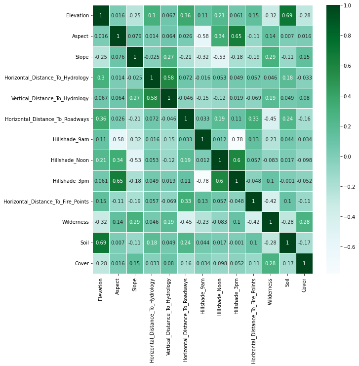
Thus, these columns will be least helpful in predicting the cover type, which is the goal of this project. Let's see if we can find out more about which features we should remove. First, note
Tree-based algorithms and feature selection
To make the next couple algorithms as efficient as possible, we can use some of the information we gathered from thetree-based classifiers to see which features are the least important in prediction. The following tables show us the features with the lowest importance values in the random forest classifier, which performed the best in our tree-based analysis. Removing those features can help us reduce noise in the later algorithms' predictions.
In [92]
feat_df = pd.DataFrame(zip(feat_rf,feat_et, feat_rf), index=[train.columns], columns= ['RF', 'ET', 'DT'])
print(feat_df.shape)
print('The following features have the least importance in the random forest classifier: \n' + str(feat_df.sort_values(by = 'RF').head(15)))
l = [np.mean(feat_rf), np.mean(feat_dt), np.mean(feat_et)]
print('Mean:' + str(np.mean(l)))
Output: 20 lines
(54, 3)
The following features have the least importance in the random forest classifier:
                   RF        ET        DT
Soil_Type15  0.000005  0.000007  0.000005
Soil_Type7   0.000010  0.000046  0.000010
Soil_Type8   0.000043  0.000052  0.000043
Soil_Type36  0.000082  0.000142  0.000082
Soil_Type9   0.000116  0.000240  0.000116
Soil_Type28  0.000165  0.000259  0.000165
Soil_Type25  0.000186  0.000371  0.000186
Soil_Type18  0.000203  0.000591  0.000203
Soil_Type14  0.000386  0.000648  0.000386
Soil_Type26  0.000419  0.000936  0.000419
Soil_Type5   0.000479  0.000724  0.000479
Soil_Type27  0.000588  0.000743  0.000588
Soil_Type34  0.000609  0.000944  0.000609
Soil_Type37  0.000629  0.000759  0.000629
Soil_Type21  0.000685  0.001148  0.000685
Mean:0.018518518518518517
The above chart displays the features previous tree-based algorithms determined were the least important. I'm interested to see how important soil type and wilderness area is overall. Let's run a new random forest without the one-hot encoding for soil type and wilderness.
In [93]
trees_tr = trees_num.drop('Cover', axis = 1)
labels_tr = trees_num['Cover']

train, test, train_labels, test_labels = train_test_split(trees_tr, labels_training, test_size=0.3, random_state=1)
rf = RandomForestClassifier()
rf.fit(train, train_labels)
rf_pred = rf.predict(test)
rf_acc = accuracy_score(rf_pred , test_labels)
feat_rf = rf.feature_importances_
print("Our random forest classified {:0.2f}% of the of the trees correctly".format(rf_acc*100))
Our random forest classified 96.11% of the of the trees correctly
It seems the one-hot encoding did create a bit of noise, because this random forest was able to classify the tree cover type much better. Let's look at the feature relevance.
In [94]
plt.figure(figsize=(10,15))
plt.barh(train.columns.values,feat_rf)
plt.title('Feature Importance for Random Forest Algorithm',fontsize=10)
plt.ylabel('Feature Name')
plt.xlabel('Relevance')
plt.show()
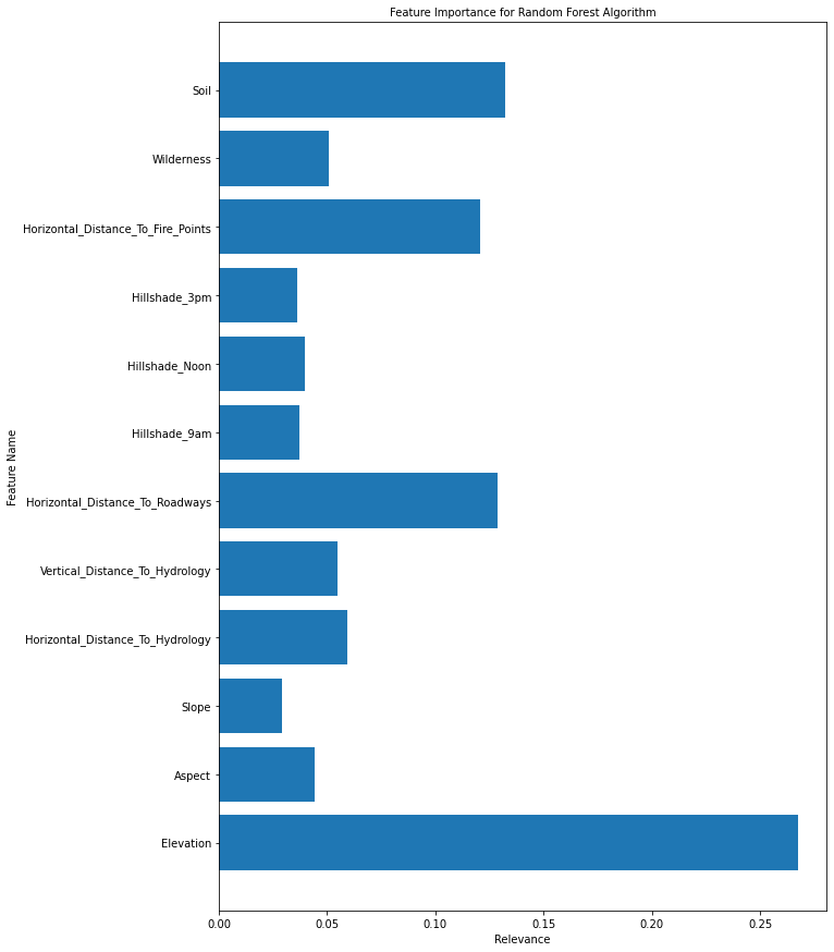
I'm going to drop the column 'Hillshade_3pm' since it is strongly corelated with the 'Hillshade_Noon' column as well as the Aspect column, but also has low relevance to the model. In addition, I will be adding some other columns related to the continuous variables:
- Euclidean distance to hydrology
- Linear combination of Elevation and Aspect
- Linear combination of Horizontal_Distance_To_Roadways and Horizontal_Distance_To_Fire_Points
- Linear combination of Horizontal_Distance_To_Roadways and Horizontal_Distance_To_Hydrology
- Linear combination of Horizontal_Distance_To_Roadways and Vertical_Distance_To_Hydrology
In addition, I'm going to normalize the Hillshade columns (in this case, divide them by 254), and perform a log transform on the Elevation and Horizontal Distance columns, as they have positive values. We will also perform square root on the Elevation and Horizontal Distance columns. This will help normalize some of those large values, and we will see the correlation and the random forest classifier feature importance to determine which features we will keep.
In [95]
df = trees_num.copy()
df['Euc_Distance_To_Hydrology'] = (trees_num['Horizontal_Distance_To_Hydrology']**2 + trees_num['Vertical_Distance_To_Hydrology']**2)**0.5
df['LC_Horizontal_Roadways_FirePoints'] = 0.5*(trees_num['Horizontal_Distance_To_Roadways'] + trees_num['Horizontal_Distance_To_Fire_Points'])
df['LC_Horizontal_Roadways_Hydrology'] = 0.5*(trees_num['Horizontal_Distance_To_Roadways'] + trees_num['Horizontal_Distance_To_Hydrology'])
df['LC_Horizontal_Roadways_Vertical_Hydrology'] = 0.5*(trees_num['Horizontal_Distance_To_Roadways'] + trees_num['Vertical_Distance_To_Hydrology'])

# Sqrt columns
df['sqrt_Elevation'] =(trees_num['Elevation'])**0.5
df['sqrt_Horizontal_Distance_To_Hydrology'] =(trees_num['Horizontal_Distance_To_Hydrology'])**0.5
df['sqrt_Horizontal_Distance_To_Roadways'] =(trees_num['Horizontal_Distance_To_Roadways'])**0.5
df['sqrt_Horizontal_Distance_To_Fire_Points'] =(trees_num['Horizontal_Distance_To_Fire_Points'])**0.5
df['sqrt_Euc_Distance_To_Hydrology'] = (df['Euc_Distance_To_Hydrology'])**0.5

# Normalize Hillshade & drop the Hillshade_3pm
df = df.drop(['Hillshade_3pm'], axis = 1)
df['norm_Hillshade_Noon'] = df['Hillshade_Noon']/254
df['norm_Hillshade_9am'] = df['Hillshade_9am']/254
df['norm_Aspect'] = df['Aspect']/360

#print(df[~df.isin([np.nan, np.inf, -np.inf]).any(1)])

print( 'Null values? :' , df.isna().any().any())


corr = df.corr()['Cover']
corr = pd.DataFrame(data =corr)
corr = corr.rename({'Cover': 'Correlation'}, axis = 1)
corr_vis = corr.abs()
print(corr_vis.sort_values(by = 'Correlation'))
Output: 27 lines
Null values? : False
                                           Correlation
norm_Aspect                                   0.015804
Aspect                                        0.015804
Euc_Distance_To_Hydrology                     0.026680
sqrt_Euc_Distance_To_Hydrology                0.032600
Horizontal_Distance_To_Hydrology              0.032768
Hillshade_9am                                 0.034286
norm_Hillshade_9am                            0.034286
sqrt_Horizontal_Distance_To_Hydrology         0.038833
Vertical_Distance_To_Hydrology                0.079644
norm_Hillshade_Noon                           0.098474
Hillshade_Noon                                0.098474
Horizontal_Distance_To_Fire_Points            0.113677
sqrt_Horizontal_Distance_To_Fire_Points       0.123971
Slope                                         0.152433
LC_Horizontal_Roadways_Vertical_Hydrology     0.159253
Horizontal_Distance_To_Roadways               0.161764
LC_Horizontal_Roadways_Hydrology              0.163136
sqrt_Horizontal_Distance_To_Roadways          0.169593
LC_Horizontal_Roadways_FirePoints             0.170957
Soil                                          0.171057
Wilderness                                    0.275180
Elevation                                     0.282160
sqrt_Elevation                                0.292478
Cover                                         1.000000
In [96]
print('Nan values?: '+str(np.any(np.isnan(df))))
print('No inf values?: '+str(np.all(np.isfinite(df))))
display(pd.DataFrame.describe(df))
display(pd.DataFrame.info(df))
Nan values?: False
No inf values?: True
| Elevation | Aspect | Slope | Horizontal_Distance_To_Hydrology | Vertical_Distance_To_Hydrology | Horizontal_Distance_To_Roadways | Hillshade_9am | Hillshade_Noon | Horizontal_Distance_To_Fire_Points | Wilderness | Soil | Cover | Euc_Distance_To_Hydrology | … | |
|---|---|---|---|---|---|---|---|---|---|---|---|---|---|---|
| count | 575348.000000 | 575348.000000 | 575348.000000 | 575348.000000 | 575348.000000 | 575348.000000 | 575348.000000 | 575348.000000 | 575348.000000 | 575348.000000 | 575348.000000 | 575348.000000 | 575348.000000 | … |
| mean | 2957.298755 | 155.361991 | 14.053832 | 264.080025 | 43.877116 | 2351.681219 | 212.312809 | 223.345940 | 1982.959816 | 2.109077 | 24.305933 | 2.047775 | 270.189276 | … |
| std | 279.109287 | 111.821993 | 7.469048 | 205.310986 | 52.303259 | 1561.492147 | 26.582840 | 19.757596 | 1328.313906 | 1.062219 | 9.473156 | 1.389914 | 208.685038 | … |
| min | 1859.000000 | 0.000000 | 0.000000 | 0.000000 | -173.000000 | 0.000000 | 0.000000 | 0.000000 | 0.000000 | 1.000000 | 1.000000 | 1.000000 | 0.000000 | … |
| 25% | 2807.000000 | 58.000000 | 9.000000 | 108.000000 | 7.000000 | 1106.000000 | 199.000000 | 213.000000 | 1022.000000 | 1.000000 | 20.000000 | 1.000000 | 108.226614 | … |
| 50% | 2995.000000 | 127.000000 | 13.000000 | 216.000000 | 29.000000 | 1998.000000 | 218.000000 | 226.000000 | 1712.000000 | 2.000000 | 29.000000 | 2.000000 | 226.901960 | … |
| 75% | 3162.000000 | 260.000000 | 18.000000 | 379.000000 | 67.000000 | 3331.000000 | 231.000000 | 237.000000 | 2552.000000 | 3.000000 | 31.000000 | 2.000000 | 389.630594 | … |
| max | 3858.000000 | 360.000000 | 66.000000 | 1211.000000 | 254.000000 | 7117.000000 | 254.000000 | 254.000000 | 7173.000000 | 4.000000 | 40.000000 | 7.000000 | 1235.336796 | … |
Showing 14 of 25 columns. Full data is in the source notebook.
Output: 32 lines
<class 'pandas.core.frame.DataFrame'>
Int64Index: 575348 entries, 0 to 581011
Data columns (total 24 columns):
 #   Column                                     Non-Null Count   Dtype
---  ------                                     --------------   -----
 0   Elevation                                  575348 non-null  int64
 1   Aspect                                     575348 non-null  int64
 2   Slope                                      575348 non-null  int64
 3   Horizontal_Distance_To_Hydrology           575348 non-null  int64
 4   Vertical_Distance_To_Hydrology             575348 non-null  int64
 5   Horizontal_Distance_To_Roadways            575348 non-null  int64
 6   Hillshade_9am                              575348 non-null  int64
 7   Hillshade_Noon                             575348 non-null  int64
 8   Horizontal_Distance_To_Fire_Points         575348 non-null  int64
 9   Wilderness                                 575348 non-null  int64
 10  Soil                                       575348 non-null  int64
 11  Cover                                      575348 non-null  int64
 12  Euc_Distance_To_Hydrology                  575348 non-null  float64
 13  LC_Horizontal_Roadways_FirePoints          575348 non-null  float64
 14  LC_Horizontal_Roadways_Hydrology           575348 non-null  float64
 15  LC_Horizontal_Roadways_Vertical_Hydrology  575348 non-null  float64
 16  sqrt_Elevation                             575348 non-null  float64
 17  sqrt_Horizontal_Distance_To_Hydrology      575348 non-null  float64
 18  sqrt_Horizontal_Distance_To_Roadways       575348 non-null  float64
 19  sqrt_Horizontal_Distance_To_Fire_Points    575348 non-null  float64
 20  sqrt_Euc_Distance_To_Hydrology             575348 non-null  float64
 21  norm_Hillshade_Noon                        575348 non-null  float64
 22  norm_Hillshade_9am                         575348 non-null  float64
 23  norm_Aspect                                575348 non-null  float64
dtypes: float64(12), int64(12)
memory usage: 125.9 MB
None
In [97]
trees_tr = df.drop('Cover', axis = 1)
labels_tr = df['Cover']

train, test, train_labels, test_labels = train_test_split(trees_tr, labels_training, test_size=0.3, random_state=1)
rf = RandomForestClassifier()
rf.fit(train, train_labels)
rf_pred = rf.predict(test)
rf_acc = accuracy_score(rf_pred , test_labels)

feat_rf_new = rf.feature_importances_
print("Our random forest classified {:0.2f}% of the of the trees correctly".format(rf_acc*100))
Our random forest classified 96.94% of the of the trees correctly
In [98]
l = pd.DataFrame(zip(train.columns.values,feat_rf_new))
print(l.sort_values(by = 1))
plt.figure(figsize=(10,15))
plt.barh(train.columns.values,feat_rf_new)
plt.title('Feature Importance for Random Forest Algorithm',fontsize=10)
plt.ylabel('Feature Name')
plt.xlabel('Relevance')
plt.show()
Output: 25 lines
                                            0         1
2                                       Slope  0.016840
3            Horizontal_Distance_To_Hydrology  0.017300
16      sqrt_Horizontal_Distance_To_Hydrology  0.018300
7                              Hillshade_Noon  0.020102
20                        norm_Hillshade_Noon  0.020357
6                               Hillshade_9am  0.020595
21                         norm_Hillshade_9am  0.020917
1                                      Aspect  0.021531
22                                norm_Aspect  0.021572
11                  Euc_Distance_To_Hydrology  0.021683
19             sqrt_Euc_Distance_To_Hydrology  0.022279
4              Vertical_Distance_To_Hydrology  0.027925
9                                  Wilderness  0.038626
14  LC_Horizontal_Roadways_Vertical_Hydrology  0.038708
5             Horizontal_Distance_To_Roadways  0.038995
17       sqrt_Horizontal_Distance_To_Roadways  0.039787
13           LC_Horizontal_Roadways_Hydrology  0.041627
18    sqrt_Horizontal_Distance_To_Fire_Points  0.054596
8          Horizontal_Distance_To_Fire_Points  0.054826
12          LC_Horizontal_Roadways_FirePoints  0.068097
10                                       Soil  0.092398
15                             sqrt_Elevation  0.141140
0                                   Elevation  0.141801
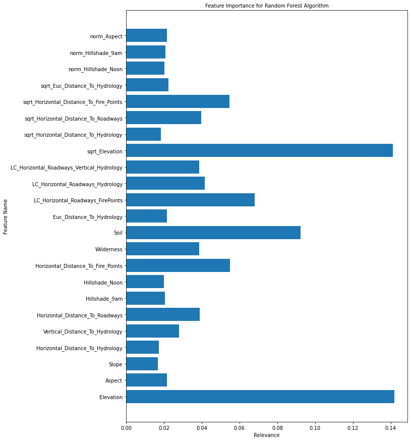
Looking at the above chart as well as the correlation to Cover Type, I'm going to drop the following columns:
- Hillshade_Noon
- Hillshade_9am
- Horizontal_Distance_To_Hydrology
- sqrt_Horizontal_Distance_To_Hydrology
- Euc_Distance_To_Hydrology
- Horizontal_Distance_To_Roadways
- Aspect
This is because other columns have a high correlation (and mututal information) with these columns, so they're redundant and will most likely create noise for our algorithms.
In [99]
df = df.drop([ 'Hillshade_Noon','Hillshade_9am','Horizontal_Distance_To_Hydrology', 'sqrt_Horizontal_Distance_To_Hydrology','Euc_Distance_To_Hydrology', 'Horizontal_Distance_To_Roadways' ,'Aspect'], axis = 1)
Let's see if there are any other columns left with very high correlation to other features.
In [100]
plt.figure(figsize=(10,10))

sns.heatmap(df.corr(),cmap='BuGn',linecolor='white',linewidths=1,annot=True, xticklabels = True, yticklabels= True)
<AxesSubplot:>
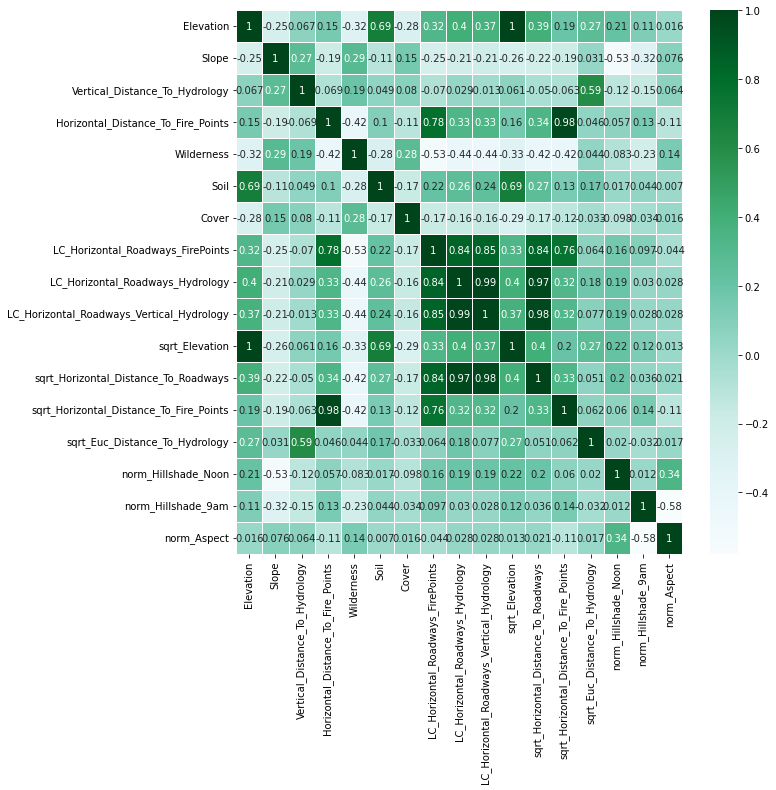
Looks like there are a couple more columns we can remove. We will remove:
- Elevation
- Horizontal_Distance_To_Fire_Points
- sqrt_Horizontal_Distance_To_Roadways
In [101]
df = df.drop([ 'sqrt_Horizontal_Distance_To_Roadways','Horizontal_Distance_To_Fire_Points' ,'Elevation', 'LC_Horizontal_Roadways_Vertical_Hydrology' ], axis = 1)
print(df.shape)
(575348, 13)
This is a good number of features, we can move on into other algorithms for prediction.
K-Nearest Neighbors (KNN)
To run some of our algorithms for classification, we will need to create a small function that can fit the model to the data, find the test accuracy, and append this info so we can visualize and compare models later. We also need to normalize the data with z-scores for some of the models, and especially K-NN, so we will do that pre-processing as well. This way, the model performs its best so we can evaluate the models.
In [102]
def fit_evaluate_model(model, X_train, y_train, X_valid, Y_valid, method_name):

    '''
    This function trains a given model, generates predictions, appends the name of the method and the accuracy to a pre-defined list; then it returns accuracy rate

    Parameters: scikit-learn model, training data, training labels, test data, test labels

    Output: none; accuracy rate is printed

    '''
    model.fit(X_train, y_train)
    y_predicted = model.predict(X_valid)
    accuracy = accuracy_score(Y_valid, y_predicted)
    acc.append(accuracy)
    algs.append(method_name)
    print("Our {} algorithm classified {:0.2f}% of the of the trees correctly".format(method_name,accuracy*100))
In [103]
trees_tr = df.drop('Cover', axis = 1)
labels_tr = df['Cover']

train, test, train_labels, test_labels = train_test_split(trees_tr, labels_training, test_size=0.3, random_state=1)

scaler = StandardScaler()

# apply normalization to training set and transform training set
train_scaled = scaler.fit_transform(train, train_labels)
train_scaled = pd.DataFrame(train_scaled)
# transform validation set
test_scaled = scaler.transform(test)
In [104]
knn = KNeighborsClassifier()
fit_evaluate_model(knn, train_scaled, train_labels, test_scaled, test_labels, 'K-NN')
Our K-NN algorithm classified 92.71% of the of the trees correctly
Light Gradient Boosting Machine (LightGBM)
In [105]
lgbm = LGBMClassifier()
fit_evaluate_model(lgbm, train, train_labels, test, test_labels, 'LightGBM')
Our Gradient Boosting Machine algorithm classified 85.64% of the of the trees correctly
Extra Gradient Boosting (XGBoost)
In [106]
xgb = XGBClassifier()
fit_evaluate_model(xgb, train_scaled, train_labels, test_scaled, test_labels, 'XGBoost')
<local path removed>\AppData\Local\Programs\Python\Python39\lib\site-packages\xgboost\sklearn.py:1146: UserWarning: The use of label encoder in XGBClassifier is deprecated and will be removed in a future release. To remove this warning, do the following: 1) Pass option use_label_encoder=False when constructing XGBClassifier object; and 2) Encode your labels (y) as integers starting with 0, i.e. 0, 1, 2, ..., [num_class - 1].
  warnings.warn(label_encoder_deprecation_msg, UserWarning)
[15:08:50] WARNING: C:<local path removed> Starting in XGBoost 1.3.0, the default evaluation metric used with the objective 'multi:softprob' was changed from 'merror' to 'mlogloss'. Explicitly set eval_metric if you'd like to restore the old behavior.
Our XGBoost algorithm classified 88.07% of the of the trees correctly
Comparing Models & Conclusion
In [115]
predictions = pd.DataFrame(zip(algs,acc), columns= ['Model', 'Accuracy'])
predictions = predictions.sort_values(by = 'Accuracy')
plt.figure(figsize=(10,10))
ax = sns.barplot(x='Accuracy', y= 'Model', data=predictions, palette='Greens')
plt.title("Prediction Accuracy of Different Models", size=14)
Text(0.5, 1.0, 'Prediction Accuracy of Different Models')
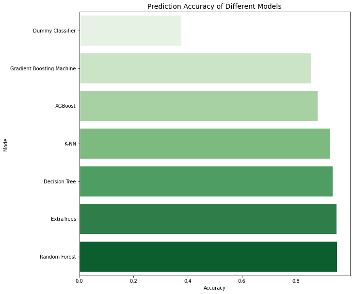
It seems the Random Forest algorithm was able to predict the tree cover most accurately. In fact, the accuracy is a bit higher for random forest after feature engineering, so random forest would be the algorithm of choice for predicting tree canopies.